Under active development. A stable version is expected in November 2026. Feedback is welcome by email or via GitHub issues.

8 Empirical Illustration: Neural Networks for Realized Volatility

8.1 Overview

Neural-network architectures are often introduced as if the main empirical question were which architecture is most powerful. In time-series econometrics, that is usually the wrong starting point. Before comparing a feed-forward network, a recurrent network, or an LSTM, we must define the forecast target, the information set at each forecast origin, the validation scheme, and the loss function used for evaluation.

This chapter makes those choices explicit in a single empirical illustration. The object is one-step-ahead forecasting of SPDR S&P 500 ETF (SPY) realized volatility, using the daily realized-variance measures described in the dataset appendix.

The empirical comparison has two purposes. First, it shows why modeling \(\log(RV)\) is often more stable than modeling realized variance in levels. Second, it compares a linear HAR-OLS benchmark with four neural-network specifications — a parsimonious HAR-FNN, a full feed-forward network, a Simple RNN, and an LSTM — all evaluated under the same forecast-origin discipline. A central finding is that HAR-OLS is hard to beat: the nonlinear HAR-FNN loses to its linear counterpart on every loss, and the full-history neural networks at best match HAR-OLS.

8.2 Roadmap

We define the realized-volatility target and the one-step-ahead forecast origin.
We specify the local-data workflow and the time-ordered train-validation-test split.
We define the HAR-OLS, HAR-FNN, full FNN, Simple RNN, and LSTM inputs.
We tune the neural networks using only the validation block.
We interpret the empirical results as evidence about target transformations, benchmark choice, and architecture choice.

8.3 Data and Forecast Target

Let \(r_{t,j}\) denote the \(j\)th intraday return on trading day \(t\). A standard realized-variance measure is

RV_t=\sum_{j=1}^{M_t} r_{t,j}^2,

where \(M_t\) is the number of intraday return intervals available after cleaning. Realized variance — the sum of intraday squared returns as a consistent estimator of integrated variance under standard semimartingale assumptions — is a canonical high-frequency volatility measure; Andersen et al. (2003) is a standard reference for modeling and forecasting it. It is positive, highly right-skewed, and persistent. For that reason, a common forecasting target is

z_t = \log(RV_t),

although the empirical comparison below also reports what happens when the networks are fit directly to \(RV_t\) in levels.

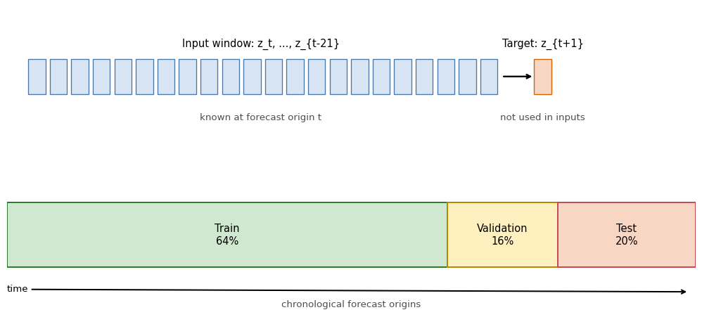
For the log target, the one-step-ahead forecasting problem is

\widehat z_{t+1\mid t} = f_\theta(z_t,z_{t-1},\ldots,z_{t-21}),

where the input window contains the previous 22 trading days, roughly one trading month. The forecast target \(z_{t+1}\) is not part of the input window.

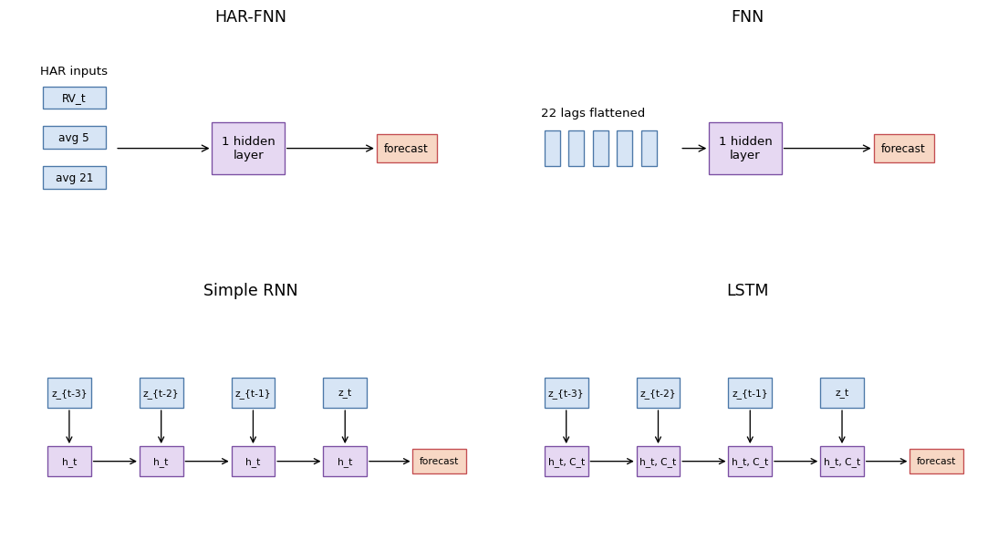
The full-history models all use this same forecast-origin history. The full FNN receives the 22 lags as a flattened feature vector. The Simple RNN and LSTM receive the same values as an ordered sequence. The HAR specifications are different by design: they receive a traditional volatility summary consisting of yesterday’s realized variance \(RV_t\), the trailing 5-day average, and the trailing 21-day average. This three-component (daily, weekly, monthly) decomposition is the heterogeneous autoregressive model of Corsi (2009), designed to capture the long-memory structure of realized volatility with a parsimonious linear specification. All three components are known at the forecast origin \(t\).

The local replication code expects the daily SPY realized-measures file documented in the dataset appendix.

Figure 8.1 shows the forecast-origin convention. The training, validation, and test blocks are chronological. Scaling constants and hyperparameters are learned before the test block is touched.

Figure 8.1: Forecast-origin convention for the volatility experiment. Each one-step-ahead forecast uses the previous 22 trading days of log realized variance. The chronological split uses the first 64% of valid forecast origins for training, the next 16% for validation and tuning, and the final 20% for test evaluation.

The workflow below makes the econometric design explicit: it constructs forecast origins before splitting the sample, estimates scaling constants only on the training block, and keeps the test block untouched until the final comparison. Replication uses the local SPY realized-variance file documented in the dataset appendix.

The first chunk loads the realized-variance series and constructs \(z_t=\log(RV_t)\). Rows with missing or nonpositive realized variance are excluded before forming forecast origins.

Show the code

import os
os.environ["KERAS_BACKEND"] = "tensorflow"
os.environ["TF_CPP_MIN_LOG_LEVEL"] = "3"

import random
import numpy as np
import pandas as pd
import optuna
import keras
from keras import layers
from sklearn.metrics import mean_absolute_error, root_mean_squared_error
from sklearn.linear_model import LinearRegression

optuna.logging.set_verbosity(optuna.logging.WARNING)
random.seed(0)
np.random.seed(0)
keras.utils.set_random_seed(0)

path = "data/taq_spy/SPY_daily_measures.csv"
rv = (
    pd.read_csv(path, parse_dates=["date"])
    .sort_values("date")
    .loc[:, ["date", "rv"]]
    .dropna()
)
rv = rv.loc[rv["rv"] > 0].reset_index(drop=True)
rv["z"] = np.log(rv["rv"])
print(f"observations: {len(rv)}, range: {rv['date'].min().date()} to {rv['date'].max().date()}")

observations: 2451, range: 2015-01-02 to 2024-12-31

The next helper constructs the supervised forecasting problem. For each valid origin \(t\), the full-history models see \((z_t,\ldots,z_{t-21})\) and forecast \(z_{t+1}\). The HAR helper uses the same origin \(t\) but replaces the 22 individual lags by three realized-variance summaries:

\left( RV_t,\quad \frac{1}{5}\sum_{j=0}^{4} RV_{t-j},\quad \frac{1}{21}\sum_{j=0}^{20} RV_{t-j} \right).

The training block is the first 64% of valid forecast origins, the validation block is the next 16%, and the test block is the final 20%. The validation block is sized to give enough forecast origins for stable hyperparameter selection via Optuna while keeping the test block large enough for a reliable out-of-sample comparison.

Show the code

window = 22

def make_windows(values, window):
    X, y, target_index = [], [], []
    for end in range(window - 1, len(values) - 1):
        X.append(values[end - window + 1 : end + 1])
        y.append(values[end + 1])
        target_index.append(end + 1)
    return np.asarray(X), np.asarray(y), np.asarray(target_index)

def make_har_features(rv_values, target_values, window):
    X, y, target_index = [], [], []
    for end in range(window - 1, len(rv_values) - 1):
        X.append(
            [
                rv_values[end],
                rv_values[end - 4 : end + 1].mean(),
                rv_values[end - 20 : end + 1].mean(),
            ]
        )
        y.append(target_values[end + 1])
        target_index.append(end + 1)
    return np.asarray(X), np.asarray(y), np.asarray(target_index)

def make_log_har_ols_features(rv_values, window):
    X, y, target_index = [], [], []
    for end in range(window - 1, len(rv_values) - 1):
        X.append(
            np.log(
                [
                    rv_values[end],
                    rv_values[end - 4 : end + 1].mean(),
                    rv_values[end - 20 : end + 1].mean(),
                ]
            )
        )
        y.append(np.log(rv_values[end + 1]))
        target_index.append(end + 1)
    return np.asarray(X), np.asarray(y), np.asarray(target_index)

X_raw, y_raw, target_index = make_windows(rv["z"].to_numpy(), window)
X_har_ols_log_raw, y_har_ols_log_raw, _ = make_log_har_ols_features(
    rv["rv"].to_numpy(),
    window,
)
X_har_raw, y_har_raw, target_index_har = make_har_features(
    rv["rv"].to_numpy(),
    rv["z"].to_numpy(),
    window,
)
X_har_rv_raw, y_har_rv_raw, _ = make_har_features(
    rv["rv"].to_numpy(),
    rv["rv"].to_numpy(),
    window,
)
X_lag_rv_raw, y_lag_rv_raw, _ = make_windows(rv["rv"].to_numpy(), window)
dates = rv.loc[target_index, "date"].reset_index(drop=True)

n = len(y_raw)
train_end = int(0.64 * n)
valid_end = int(0.80 * n)

X_train_raw, y_train_raw = X_raw[:train_end], y_raw[:train_end]
X_valid_raw, y_valid_raw = X_raw[train_end:valid_end], y_raw[train_end:valid_end]
X_test_raw, y_test = X_raw[valid_end:], y_raw[valid_end:]
test_dates = dates.iloc[valid_end:].reset_index(drop=True)

X_har_train_raw = X_har_raw[:train_end]
X_har_valid_raw = X_har_raw[train_end:valid_end]
X_har_test_raw = X_har_raw[valid_end:]

X_har_ols_log_train_valid_raw = X_har_ols_log_raw[:valid_end]
X_har_ols_log_test_raw = X_har_ols_log_raw[valid_end:]
y_har_ols_log_train_valid = y_har_ols_log_raw[:valid_end]

X_har_rv_train_raw = X_har_rv_raw[:train_end]
X_har_rv_valid_raw = X_har_rv_raw[train_end:valid_end]
X_har_rv_test_raw = X_har_rv_raw[valid_end:]
y_rv_train_raw = y_har_rv_raw[:train_end]
y_rv_valid_raw = y_har_rv_raw[train_end:valid_end]
y_rv_test = y_har_rv_raw[valid_end:]
X_har_ols_rv_train_valid_raw = X_har_rv_raw[:valid_end]
X_har_ols_rv_test_raw = X_har_rv_raw[valid_end:]
y_har_ols_rv_train_valid = y_har_rv_raw[:valid_end]

X_lag_rv_train_raw = X_lag_rv_raw[:train_end]
X_lag_rv_valid_raw = X_lag_rv_raw[train_end:valid_end]
X_lag_rv_test_raw = X_lag_rv_raw[valid_end:]

center = y_train_raw.mean()
scale = y_train_raw.std()
x_har_center = X_har_train_raw.mean(axis=0)
x_har_scale = X_har_train_raw.std(axis=0)
x_har_scale = np.where(x_har_scale == 0, 1, x_har_scale)

x_har_rv_center = X_har_rv_train_raw.mean(axis=0)
x_har_rv_scale = X_har_rv_train_raw.std(axis=0)
x_har_rv_scale = np.where(x_har_rv_scale == 0, 1, x_har_rv_scale)
y_rv_center = y_rv_train_raw.mean()
y_rv_scale = y_rv_train_raw.std()

x_lag_rv_center = X_lag_rv_train_raw.mean(axis=0)
x_lag_rv_scale = X_lag_rv_train_raw.std(axis=0)
x_lag_rv_scale = np.where(x_lag_rv_scale == 0, 1, x_lag_rv_scale)

def standardize(a):
    return (a - center) / scale

def unstandardize(a):
    return a * scale + center

def standardize_har(a):
    return (a - x_har_center) / x_har_scale

def standardize_har_rv(a):
    return (a - x_har_rv_center) / x_har_rv_scale

def unstandardize_rv(a):
    return a * y_rv_scale + y_rv_center

def standardize_lag_rv(a):
    return (a - x_lag_rv_center) / x_lag_rv_scale

X_train = standardize(X_train_raw)
X_valid = standardize(X_valid_raw)
X_test = standardize(X_test_raw)
X_har_train = standardize_har(X_har_train_raw)
X_har_valid = standardize_har(X_har_valid_raw)
X_har_test = standardize_har(X_har_test_raw)
y_train = standardize(y_train_raw)
y_valid = standardize(y_valid_raw)

X_har_rv_train = standardize_har_rv(X_har_rv_train_raw)
X_har_rv_valid = standardize_har_rv(X_har_rv_valid_raw)
X_har_rv_test = standardize_har_rv(X_har_rv_test_raw)
y_rv_train = (y_rv_train_raw - y_rv_center) / y_rv_scale
y_rv_valid = (y_rv_valid_raw - y_rv_center) / y_rv_scale

X_lag_rv_train = standardize_lag_rv(X_lag_rv_train_raw)
X_lag_rv_valid = standardize_lag_rv(X_lag_rv_valid_raw)
X_lag_rv_test = standardize_lag_rv(X_lag_rv_test_raw)

print(f"forecast origins: {n}")
print(f"train: {train_end}, validation: {valid_end - train_end}, test: {n - valid_end}")

forecast origins: 2429
train: 1554, validation: 389, test: 486

8.4 Comparable Specifications

The specifications differ in how they represent the same forecasting problem.

The HAR-OLS benchmark is linear. For the log target, it regresses \(\log(RV_{t+1})\) on the logs of the daily, weekly, and monthly HAR components. For the level target, it regresses \(RV_{t+1}\) on the corresponding level components.
The HAR-FNN is the most structured specification. It uses the three HAR volatility-component summaries — daily, weekly, and monthly averages of realized variance — that follow the Corsi (2009) model.
The full FNN uses the full 22-day history but treats it as an unordered vector of features.
The Simple RNN also uses the full 22-day history, but processes the lags sequentially through a recurrent state.
The LSTM processes the same sequence with gated memory, allowing the network to regulate how much past information is retained.

Figure 8.2 summarizes the neural specifications. The models differ in input representation, not in parameter count, and the information available at forecast origin \(t\) is held fixed and documented across architectures. HAR-OLS is included because the nonlinear HAR-FNN is informative only as a comparison against the linear HAR model it generalizes.

All four neural networks are deliberately shallow. The HAR-FNN and full FNN have one hidden dense layer with a tuned width and a linear output layer. The Simple RNN and LSTM have one recurrent layer with a tuned number of units and a linear output layer. A deeper pyramidal FNN, for example 22 inputs to 64 hidden units to 32 hidden units to one output, would be a reasonable robustness check. It is not the baseline here because it would add another capacity choice while the chapter’s main comparison is about target transformation and information representation.

Figure 8.2: Four volatility-forecasting specifications. The HAR-FNN uses yesterday’s realized variance, the trailing 5-day average, and the trailing 21-day average. The full FNN flattens the 22-day window. The Simple RNN and LSTM process the ordered sequence.

Each architecture below uses the same skeleton — one hidden layer of tuned width followed by a linear output. The input shapes enforce the intended information sets: three HAR features for the HAR-FNN, 22 flattened lags for the full FNN, and a 22-step sequence for the recurrent models.

Show the code

def make_fnn(n_neurons, learning_rate):
    model = keras.Sequential(
        [
            keras.Input(shape=(window,)),
            layers.Dense(n_neurons, activation="softplus"),
            layers.Dense(1),
        ],
        name="FNN",
    )
    model.compile(
        loss=keras.losses.MeanSquaredError(),
        optimizer=keras.optimizers.Adam(learning_rate=learning_rate),
    )
    return model

def make_har_fnn(n_neurons, learning_rate):
    model = keras.Sequential(
        [
            keras.Input(shape=(3,)),
            layers.Dense(n_neurons, activation="softplus"),
            layers.Dense(1),
        ],
        name="HARFNN",
    )
    model.compile(
        loss=keras.losses.MeanSquaredError(),
        optimizer=keras.optimizers.Adam(learning_rate=learning_rate),
    )
    return model

def make_simple_rnn(n_neurons, learning_rate):
    model = keras.Sequential(
        [
            keras.Input(shape=(window, 1)),
            layers.SimpleRNN(n_neurons, activation="softplus", return_sequences=False),
            layers.Dense(1),
        ],
        name="SimpleRNN",
    )
    model.compile(
        loss=keras.losses.MeanSquaredError(),
        optimizer=keras.optimizers.Adam(learning_rate=learning_rate),
    )
    return model

def make_lstm(n_neurons, learning_rate):
    model = keras.Sequential(
        [
            keras.Input(shape=(window, 1)),
            layers.LSTM(n_neurons, activation="softplus", return_sequences=False),
            layers.Dense(1),
        ],
        name="LSTM",
    )
    model.compile(
        loss=keras.losses.MeanSquaredError(),
        optimizer=keras.optimizers.Adam(learning_rate=learning_rate),
    )
    return model

8.5 Validation and Tuning

Hyperparameters are selected using the validation block, not the test block. This is not a nested evaluation design; it is a compact empirical illustration with a single holdout test period. The validation block is used for model selection, and the final test block is used once after the selected hyperparameters have been fixed.

The important time-series restriction is shuffle=False. This chapter does not use random \(K\)-fold cross-validation. Random folds would mix volatility regimes across training and validation sets and would therefore no longer mimic the one-step-ahead forecasting problem.

Show the code

def as_sequence(X):
    return X[..., np.newaxis]

def tune_model(model_factory, X_tr, X_va, n_trials=20):
    def objective(trial):
        params = {
            "learning_rate": trial.suggest_float("learning_rate", 1e-4, 1e-3, log=True),
            "batch_size": trial.suggest_int("batch_size", 16, 64, step=4),
            "n_neurons": trial.suggest_int("n_neurons", 16, 96, step=4),
            "epochs": 30,
        }
        model = model_factory(params["n_neurons"], params["learning_rate"])
        history = model.fit(
            X_tr,
            y_train,
            validation_data=(X_va, y_valid),
            epochs=params["epochs"],
            batch_size=params["batch_size"],
            verbose=0,
            shuffle=False,
        )
        return min(history.history["val_loss"])

    study = optuna.create_study(
        direction="minimize",
        sampler=optuna.samplers.TPESampler(seed=1),
    )
    study.optimize(objective, n_trials=n_trials)
    return study.best_params

best_har_fnn = tune_model(make_har_fnn, X_har_train, X_har_valid)
best_fnn = tune_model(make_fnn, X_train, X_valid)
best_rnn = tune_model(make_simple_rnn, as_sequence(X_train), as_sequence(X_valid))
best_lstm = tune_model(make_lstm, as_sequence(X_train), as_sequence(X_valid))

In the local run that produced this chapter’s output, chronological validation selected the following hyperparameters. Validation losses are comparable within a target scale but not across the log(rv) and rv panels, because the training targets have different units and variances.

HAR-OLS does not appear in this table because it has no neural tuning parameters. It is fit by ordinary least squares on the combined train-validation block before the final test evaluation.

Target fit	Model	Tuned width	Learning rate	Batch size	Validation loss
`log(rv)`	HAR-FNN	72	0.000930	32	0.3643
`log(rv)`	FNN	60	0.000656	32	0.2745
`log(rv)`	Simple RNN	40	0.000318	28	0.2725
`log(rv)`	LSTM	60	0.000468	36	0.2740
`rv`	HAR-FNN	36	0.000664	44	0.0973
`rv`	FNN	36	0.000497	28	0.1009
`rv`	Simple RNN	80	0.000365	44	0.0959
`rv`	LSTM	72	0.000930	32	0.0959

The log-target full-history models have similar validation losses, so the final test comparison should not be read as a decisive ranking of recurrent memory versus a flattened lag vector. The level-target validation losses also cluster tightly. This is a useful warning: validation loss alone does not settle the target-transformation question because each panel is fit and scaled on a different target.

After tuning, each selected model is refit on the combined train-validation block and evaluated once on the test block. This gives the final table a simple interpretation: each row is the out-of-sample performance of one target choice and one architecture under the same chronological split.

Show the code

def qlike(rv_true, rv_pred):
    rv_pred = np.maximum(rv_pred, 1e-12)
    return np.mean(rv_true / rv_pred - np.log(rv_true / rv_pred) - 1)

def summarize_forecast(name, target, z_hat, rv_hat):
    rv_true = np.exp(y_test)
    z_for_log_loss = np.log(np.maximum(rv_hat, 1e-12))
    return {
        "target": target,
        "model": name,
        "rmse_log_rv": root_mean_squared_error(y_test, z_for_log_loss),
        "mae_log_rv": mean_absolute_error(y_test, z_for_log_loss),
        "rmse_rv": root_mean_squared_error(rv_true, rv_hat),
        "mae_rv": mean_absolute_error(rv_true, rv_hat),
        "qlike": qlike(rv_true, rv_hat),
        "nonpositive_rv_forecasts": int(np.sum(rv_hat <= 0)),
        "forecast": z_hat,
    }

def fit_har_ols_log():
    model = LinearRegression().fit(
        X_har_ols_log_train_valid_raw,
        y_har_ols_log_train_valid,
    )
    z_hat = model.predict(X_har_ols_log_test_raw)
    return summarize_forecast("HAR-OLS", "log(rv)", z_hat, np.exp(z_hat))

def fit_har_ols_level():
    model = LinearRegression().fit(
        X_har_ols_rv_train_valid_raw,
        y_har_ols_rv_train_valid,
    )
    rv_hat = model.predict(X_har_ols_rv_test_raw)
    z_hat = np.log(np.maximum(rv_hat, 1e-12))
    return summarize_forecast("HAR-OLS", "rv", z_hat, rv_hat)

def fit_and_score(name, model_factory, params, X_trva, y_trva, X_te):
    model = model_factory(params["n_neurons"], params["learning_rate"])
    model.fit(
        X_trva,
        y_trva,
        epochs=100,
        batch_size=params["batch_size"],
        verbose=0,
        shuffle=False,
    )
    z_hat = unstandardize(model.predict(X_te).ravel())
    rv_hat = np.exp(z_hat)
    return summarize_forecast(name, "log(rv)", z_hat, rv_hat)

X_train_valid = np.vstack([X_train, X_valid])
X_har_train_valid = np.vstack([X_har_train, X_har_valid])
y_train_valid = np.concatenate([y_train, y_valid])

results = [
    fit_har_ols_log(),
    fit_and_score("HAR-FNN", make_har_fnn, best_har_fnn, X_har_train_valid, y_train_valid, X_har_test),
    fit_and_score("FNN", make_fnn, best_fnn, X_train_valid, y_train_valid, X_test),
    fit_and_score("Simple RNN", make_simple_rnn, best_rnn, as_sequence(X_train_valid), y_train_valid, as_sequence(X_test)),
    fit_and_score("LSTM", make_lstm, best_lstm, as_sequence(X_train_valid), y_train_valid, as_sequence(X_test)),
    fit_har_ols_level(),
]

performance = pd.DataFrame(results).drop(columns=["forecast"])
performance

8.6 Results

The model-fitting and tuning code above is shown for exposition but is not executed on render; the results below come from a local run with WRDS TAQ access. The empirical output uses the SPY realized-variance file described in the dataset appendix, filtered to positive realized-variance observations; the usable modeling sample ends on 2024-12-31. The log-target rows come from the workflow shown above. The level-target rows repeat the same split, input construction, tuning budget, and evaluation protocol, but fit the models to \(RV_{t+1}\) rather than \(\log(RV_{t+1})\). The tuning run used 20 Optuna trials for each neural architecture. Figure 8.3 is likewise a pre-generated figure from the same local run.

The columns answer different questions. RMSE on \(\log(RV)\) evaluates forecasts on the scale used by the log-target models and is the main comparison criterion here. For level-target models, the log-scale metrics are computed after clipping nonpositive variance forecasts to a small positive number before taking logs. RMSE on \(RV\) evaluates the implied variance forecasts after exponentiating log-target forecasts. QLIKE is the volatility loss

\frac{1}{n_{\text{test}}}\sum_{t} \left( \frac{RV_t}{\widehat{RV}_t} - \log\frac{RV_t}{\widehat{RV}_t} -1 \right),

which is defined only for positive variance forecasts. All three measures are losses, so smaller values are better.

Target fit	Model	RMSE log RV	RMSE RV	QLIKE
`log(rv)`	HAR-OLS	0.5992	0.4121	0.2124
`log(rv)`	HAR-FNN	0.6258	0.4717	0.2367
`log(rv)`	FNN	0.6039	0.4108	0.2002
`log(rv)`	Simple RNN	0.6001	0.4118	0.2093
`log(rv)`	LSTM	0.5989	0.4120	0.2099
`rv`	HAR-OLS	0.6755	0.4197	0.1985
`rv`	HAR-FNN	0.7055	0.4372	0.2048
`rv`	FNN	0.6942	0.4506	0.2335
`rv`	Simple RNN	0.6362	0.4198	0.1916
`rv`	LSTM	0.7078	0.4364	0.2068

The next table records whether a level-target model produced nonpositive variance forecasts. In this run none did. The diagnostic is still worth reporting because a negative variance forecast has no volatility interpretation, and QLIKE must be computed only after clipping such forecasts away from zero.

Target fit	Model	Nonpositive RV forecasts
`log(rv)`	HAR-OLS	0
`log(rv)`	HAR-FNN	0
`log(rv)`	FNN	0
`log(rv)`	Simple RNN	0
`log(rv)`	LSTM	0
`rv`	HAR-OLS	0
`rv`	HAR-FNN	0
`rv`	FNN	0
`rv`	Simple RNN	0
`rv`	LSTM	0

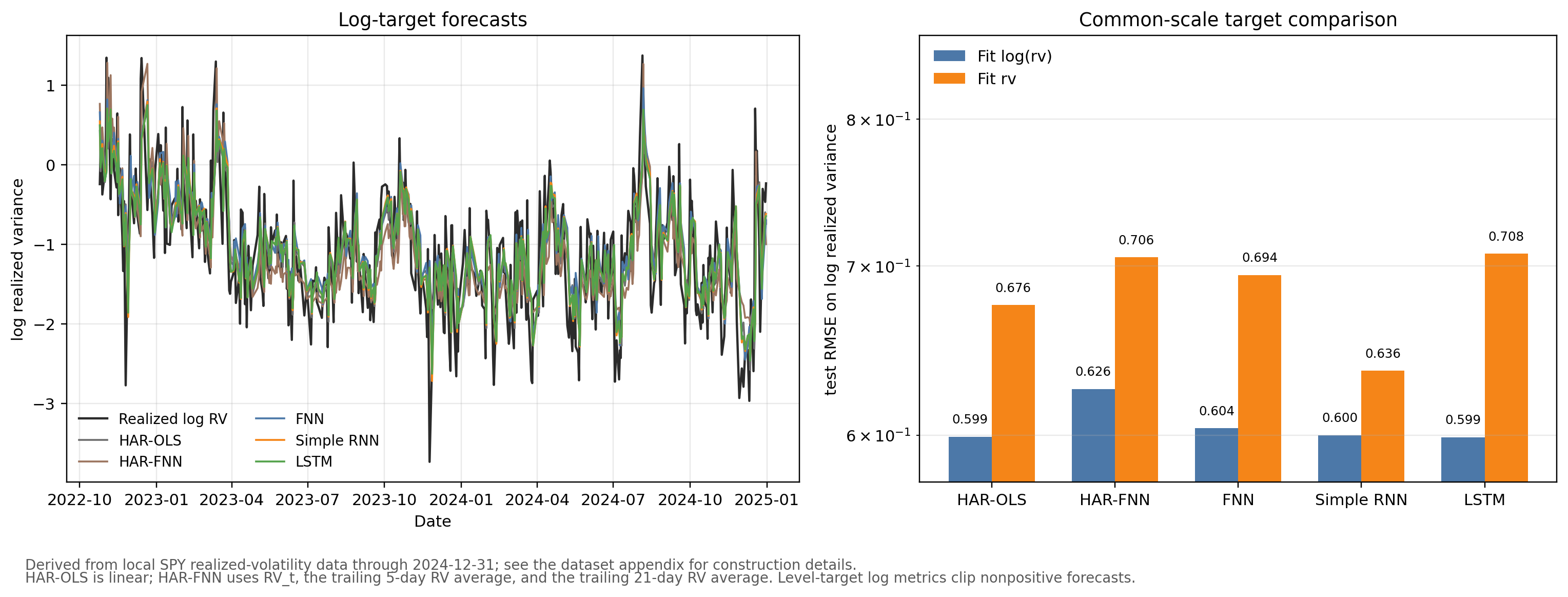
Figure 8.3: Derived empirical output from the local SPY realized-variance run. The left panel shows test-period realized log realized variance and log-target forecasts, including HAR-OLS and the three-input HAR-FNN. The right panel compares models fit on `log(rv)` with models fit on `rv`, using test RMSE on log realized variance as a common scale; the vertical axis is logarithmic.

Figure 8.3 makes the transformation choice visible. On the common log-realized-variance scale, the LSTM is the best-performing model, but its RMSE advantage over HAR-OLS is 0.0003 log-RV units — a difference that is economically negligible. HAR-OLS essentially matches the full FNN and Simple RNN as well. That is the main benchmark lesson: the neural networks are not automatically better just because they are more flexible. The level-target rows are well-behaved in this updated run, but they generally lose accuracy on the log-realized-variance scale.

Two notes on reading these rankings. First, the single test window contains a few hundred forecast origins, so the standard error of any per-model loss average is non-negligible: differences smaller than the standard deviation of the per-period squared-error differences should be read as ties. The 0.0003 log-RV-unit LSTM-versus-HAR-OLS gap is well within that band. A Diebold and Mariano (1995) test would formalize this, with a HAC variance under serial dependence in the loss differential; we omit it here to keep the chapter compact, but readers replicating the experiment should not interpret RMSE differences below roughly 0.01 as robust to test-window resampling. Second, the QLIKE column in the table above is the Patton (2011) quasi-likelihood loss for volatility, which is the standard convex robust loss in the high-frequency volatility-forecasting literature.

The two HAR rows help separate information design from neural nonlinearity. In the log-target panel, linear HAR-OLS is stronger than the HAR-FNN and nearly matches the full-history networks. In the level-target panel, HAR-OLS is stronger than the HAR-FNN on all three reported losses. For this sample, the nonlinear HAR-FNN does not improve on the linear HAR benchmark.

QLIKE and log-RV RMSE also need not pick the same winner. QLIKE is scale-equivariant: it measures whether \(\widehat{RV}_t\) tracks \(RV_t\) accurately in ratio terms, and it penalizes underprediction more heavily than overprediction through the ratio \(RV_t/\widehat{RV}_t\). A model that calibrates the relative size of volatility spikes well can win on QLIKE while losing on log-RV RMSE — which is why the Simple RNN fit in levels has the lowest QLIKE while the LSTM fit on \(\log(RV)\) has the lowest log-RV RMSE.

With dependent financial data, an architecture comparison is interpretable only after the forecast target, lag construction, scaling, validation block, and tuning protocol have been fixed. The numerical ranking of LSTM, HAR-OLS, and the FNN is secondary to that design discipline.

8.7 Summary

Key Takeaways

Empirical architecture comparisons must hold the forecast target, information set, preprocessing, validation design, and tuning budget fixed.
HAR-OLS is a strong baseline: neural networks must beat it before their added flexibility is empirically useful.
In this volatility example, modeling \(\log(RV_{t+1})\) gives the best log-scale accuracy, while level-target models can still be competitive under variance-scale losses.
Adding a nonlinear hidden layer to HAR inputs (HAR-FNN) does not improve on linear HAR-OLS in this sample; the binding constraint is the choice of input features, not linearity.
The neural networks are intentionally shallow: one hidden or recurrent layer plus a linear output layer.
Time-ordered validation is required because random splits would leak future volatility regimes into tuning.
Small architecture differences should be interpreted as predictive evidence for this design, not as structural evidence that one architecture captures an economic mechanism.

Common Pitfalls

Scaling the full volatility series before the train-validation-test split.
Skipping the linear HAR-OLS baseline and attributing gains to neural nonlinearity.
Giving the RNN or LSTM a longer history than the FNN and then attributing the gain to recurrence.
Accidentally computing HAR averages with the forecast target day included.
Treating a deeper pyramidal FNN as directly comparable without acknowledging the extra capacity choice.
Using Keras’s validation_split mechanically when it does not match the desired chronological validation block.
Shuffling observations during training or validation for a time-series forecast.
Modeling realized variance in levels and forgetting to check whether neural-network forecasts become nonpositive.

8.8 References

Andersen, Torben G., Tim Bollerslev, Francis X. Diebold, and Paul Labys. 2003. “Modeling and Forecasting Realized Volatility.” Econometrica 71 (2): 579–625. https://doi.org/10.1111/1468-0262.00418.

Corsi, Fulvio. 2009. “A Simple Approximate Long-Memory Model of Realized Volatility.” Journal of Financial Econometrics 7 (2): 174–96. https://doi.org/10.1093/jjfinec/nbp001.

Diebold, Francis X, and Robert S Mariano. 1995. “Comparing predictive accuracy.” Journal of Business and Economic Statistics 13 (3): 253–63. https://doi.org/10.1080/07350015.1995.10524599.

Patton, Andrew J. 2011. “Volatility Forecast Comparison Using Imperfect Volatility Proxies.” Journal of Econometrics 160 (1): 246–56. https://doi.org/10.1016/j.jeconom.2010.03.034.