Under active development. A stable version is expected in November 2026. Feedback is welcome by email or via GitHub issues.
Data Sets Used in This Book
17 Data Sets Used in This Book
This chapter is a reference appendix for the file-backed datasets shipped with the book repository. Earlier chapters link here instead of re-describing the source each time. Synthetic datasets generated inside code chunks are not listed here; they are documented where they appear.
17.1 FRED-QD
FRED-QD is the quarterly U.S. macroeconomic database developed by McCracken and Ng (2020). A repository copy of the release used in these notes is stored at data/fred_qd_current.csv.
Unit of observation: calendar quarter
Coverage: U.S. macro-financial series, 1959Q1 onward
Frequency: quarterly
File layout: the CSV contains two metadata rows before the actual data. The first row stores factor-group identifiers and the second row stores the authors’ suggested transformation codes. The sasdate column holds the end-of-quarter date.
The chapters in the book use the subset of series listed below. Full variable documentation is available in the FRED-QD release notes.
Mnemonic
Description
GDPC1
Real gross domestic product, chained dollars
CPIAUCSL
Consumer price index, all urban consumers
UNRATE
Civilian unemployment rate
FEDFUNDS
Effective federal funds rate
GS10
10-year Treasury constant-maturity yield
TB3MS
3-month Treasury bill secondary-market rate
VIXCLSx
CBOE volatility index (VIX), quarterly closing value
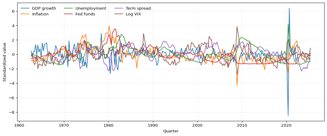
Figure 17.1 shows the series used in the book on a common standardized scale so that their timing can be compared across the sample. Magnitudes are not directly comparable on this scale.
Figure 17.1: Selected FRED-QD series used in the book, standardized to mean zero and variance one. Real GDP growth is the annualized log difference of GDPC1; inflation is the annualized log difference of CPIAUCSL; the remaining series are shown as levels, with the term spread constructed as GS10 - TB3MS and log VIX as log(VIXCLSx).
17.2 Loading FRED-QD
The snippet below is the canonical way to load FRED-QD in this book. It skips the two metadata rows, parses sasdate as a date, and coerces the remaining columns to numeric.
The authors’ transformation codes in the second metadata row are not applied here. Individual chapters construct the transformations they need directly from the raw levels so that the forecast origin and information set are explicit.
17.3 SPY TAQ 5-Minute Realized Measures
The repository also contains scripts for constructing realized-volatility measures from WRDS TAQ millisecond trade data for the SPDR S&P 500 ETF (SPY). The raw TAQ data and derived realized-measure files are not shipped with the public book because TAQ access is licensed through WRDS. The expected local paths are data/taq_spy/SPY_daily_measures.csv for the daily CSV used in the neural-network illustration and data/taq_spy/SPY_5min_daily_rv.parquet for the Parquet output produced by the 5-minute compilation script. The whole data/taq_spy/ directory is excluded from git.
Unit of observation: trading day
Underlying data: WRDS TAQ millisecond trades, queried from taqmsec.ctm_YYYYMMDD
Instrument: SPY
Frequency used for realized measures: 5-minute intraday prices
Coverage: 2015-01-02 through 2024-12-31
Construction scripts: scripts/download_spy_taq_wrds.R downloads and cleans TAQ trades; scripts/compile_spy_5min_rv_parquet.R compiles daily realized measures from the local 5-minute bar files.
The two local files have different column sets.
Daily CSV (SPY_daily_measures.csv) — used by the neural-network illustration chapter:
Variable
Description
date
Trading day
rv
Realized variance, sum of squared 5-minute log returns in percent
Parquet file (SPY_5min_daily_rv.parquet) — output of the 5-minute compilation script:
Variable
Description
date
Trading day
rv_5min
Realized variance, sum of squared 5-minute log returns in percent
bv_5min
Bipower variation, computed from adjacent absolute 5-minute returns with the standard \(\pi/2\) scaling, on the same percent (variance) scale as rv_5min
rq_5min
Realized quarticity proxy based on fourth powers of 5-minute returns, a fourth-moment (percent-to-the-fourth) quantity on the corresponding scale
McCracken, Michael W., and Serena Ng. 2020. “FRED-QD: A Quarterly Database for Macroeconomic Research.” Working Paper 26872. National Bureau of Economic Research.