Under active development. A stable version is expected in November 2026. Feedback is welcome by email or via GitHub issues.

13 Advanced Tree-Based Methods

13.1 Overview

The previous chapters treated trees, random forests, and gradient boosting mainly as tools for conditional-mean or conditional-event-probability prediction. In many econometric applications, that is not enough. A risk manager may need conditional quantiles of future losses, a central bank may care about the probability of extreme inflation outcomes, and an asset-pricing application may require a full predictive distribution rather than a point forecast.

This chapter extends tree-based methods in that direction. We focus on two ideas:

• Quantile Regression Forests (QRF), which reuse random-forest neighborhoods to estimate conditional distributions nonparametrically (Meinshausen 2006)
• Natural Gradient Boosting (NGBoost), which extends boosting to parametric predictive distributions and updates their parameters with gradients rescaled by local statistical information (Duan et al. 2020)

The chapter remains predictive rather than structural: it does not estimate causal effects, and it does not cover forests that solve general local estimating equations or replace leaf constants with local slopes (Athey, Tibshirani, and Wager 2019).

13.2 Roadmap

1. We start from the standard random-forest weight representation and use it to diagnose what ordinary forests do and do not provide.
2. We then define QRF through weighted empirical cumulative distribution functions (CDFs) and leaf-neighbor outcomes.
3. Next we introduce NGBoost as a boosted-tree method for fitting the parameters of a conditional distribution.
4. We explain the role of Fisher information, natural gradients, and constrained parameterizations.
5. We close with a comparison, summary, pitfalls, and exercises.

13.3 Standard Forests as Weighted Averages

Recall from the random-forest weight representation that a forest prediction can be read as a weighted average of training outcomes that frequently land in the same leaves as the forecast point. For a forest of B trees trained on N observations, let L_b(x) denote the terminal leaf reached by x in tree b, and let N_b(x) be the number of original training observations assigned to that leaf. The original-observation convention used by QRF defines the neighborhood mean

\hat \mu_w(x) = \sum_{i=1}^N w_i(x)y_i, \qquad w_i(x) = \frac{1}{B}\sum_{b=1}^B \frac{\mathbf{1}\{x_i \in L_b(x)\}}{N_b(x)}.

This representation is a useful way to read a forest. The weights w_i(x) define a local neighborhood around x, but the neighborhood is learned by recursive splits rather than fixed by Euclidean distance.

One convention needs stating, because it differs from the exact bagged-forest representation in the random forests chapter. Reproducing a bagged tree’s stored leaf mean requires tracking how often each observation was drawn into that tree’s bootstrap sample. The weights above instead run over the N original observations and ask whether observation i falls into the leaf region reached by x, without counting bootstrap multiplicities. This is the QRF convention introduced by Meinshausen (2006), and it is the convention used by the estimator and code below. The two conventions coincide when each tree is grown on the full original sample; with bootstrap sampling they describe the same learned partition but need not produce exactly the same conditional-mean prediction.

Why This Matters

The weight view separates two ingredients:

1. the forest learns which training observations are local neighbors of x
2. the prediction rule decides what to do with the outcomes of those neighbors

A standard random forest uses those neighbors to estimate a conditional mean. QRF uses the original-observation neighbors to estimate a conditional distribution.

13.4 Limitations of Standard Random Forests

The weighted-average view also makes the limitations of ordinary forests clear.

Only a point prediction. A standard regression forest returns an average of training outcomes in forest-defined neighborhoods. Under squared-error risk and conditions that make this weighted average consistent, its population target is the conditional mean \mathbb{E}[Y\mid X=x]. It does not directly report tail probabilities, quantiles, skewness, or multimodality of Y\mid X=x.

Constant local model. Inside each leaf, the local prediction is an average. The leaf therefore cannot represent a within-neighborhood slope even when the regression function is locally smooth rather than locally constant.

Prediction, not causality. The forest neighborhood is chosen to improve prediction. A split or variable importance measure should not be interpreted as a treatment effect or structural parameter without an identification design.

Potential honesty problem. A split is honest when the data used to choose the split structure and the data used to estimate the leaf values are disjoint. Standard forests often use the same observations for both tasks. The resulting adaptivity can bias leaf estimates because the prediction rule reuses outcomes that helped select the splits (Wager and Athey 2018).

13.5 Quantile Regression Forests as Distributional Forests

A distributional forest returns an estimated conditional distribution rather than only a point prediction. We use that phrase descriptively; the specific estimator developed here is QRF. QRF keeps the forest neighborhood idea but changes the object estimated from the neighbors. Instead of reporting only

\sum_{i=1}^N w_i(x)y_i,

it estimates the conditional CDF

\hat F(y\mid X=x) = \sum_{i=1}^N w_i(x)\mathbf{1}\{y_i \leq y\}.

This is a weighted empirical distribution of the training outcomes. Once we have \hat F(y\mid X=x), we can compute conditional medians, nominal prediction intervals, lower-tail probabilities, and other distributional functionals. A band formed from fitted quantiles is nominal because its realized coverage must still be checked on suitable out-of-sample data; QRF alone does not supply a finite-sample coverage guarantee.

QRF focuses on conditional quantiles. For a probability level \alpha\in(0,1), the estimated conditional quantile is

\widehat{q}_{\alpha}(x) = \inf\{y:\hat F(y\mid X=x)\geq \alpha\}.

An approximately equivalent implementation view is to collect the training outcomes that share terminal leaves with x across the forest, keep repeated appearances when an observation is a neighbor in multiple trees, and compute empirical quantiles of that pooled neighbor sample. The two views coincide exactly only when the leaf containing x has the same number of observations in every tree: under the weight representation, an appearance in tree b carries weight \frac{1}{B}\cdot\frac{1}{N_b(x)}, whereas in the pooled sample every appearance counts equally. Pooling therefore overweights observations that arrive through large leaves whenever leaf sizes differ across trees.

Consistency of \hat F(y\mid X=x)

Consistency of the weighted empirical CDF \hat F(y\mid X=x) requires more than the bagging logic of Chapter 11. The classical QRF theorem of Meinshausen (2006) assumes independent and identically distributed (i.i.d.) observations and a fixed predictor dimension. Under that sampling setup, it establishes, for each fixed x,

\sup_y\left|\hat{F}(y\mid X=x)-F(y\mid X=x)\right|\overset{p}{\longrightarrow}0.

The convergence is pointwise in x and uniform in the outcome threshold y. Its other conditions include a predictor density that is bounded above and bounded away from zero on its support, leaf sizes that grow while remaining a vanishing fraction of the sample, a positive probability of splitting on every predictor with sufficiently balanced child nodes, and a conditional CDF that is Lipschitz in x. A strictly increasing conditional CDF is additionally used to transfer consistency of the CDF estimator to its conditional quantiles. These assumptions make the bias–variance logic explicit: neighborhoods must shrink in predictor space, yet contain increasingly many observations. Temporal, spatial, or clustered dependence requires a separate consistency argument; time-ordered validation alone does not extend the theorem.

Honest-forest inference is related but distinct. Wager and Athey (2018) establish asymptotic normality for honest regression and causal forests, while Athey, Tibshirani, and Wager (2019) extend the framework to local moment estimators, including conditional quantiles. Those inferential results use subsampling, honesty, and additional regularity conditions; they are not a drop-in theorem for every QRF implementation.

The practical distinction matters. Bootstrap sampling is part of the original QRF construction, so bootstrap use alone does not invalidate the classical consistency argument. The default RandomForestRegressor, however, permits leaves with one observation and need not satisfy the growing-leaf or balanced-split conditions. Reusing it to construct QRF weights can yield useful empirical predictions, but out-of-sample performance does not by itself supply either the classical pointwise consistency guarantee or honest-forest inference.

Question for Reflection

Why can two forests with the same conditional-mean prediction still give different conditional quantile estimates?

Suggested Answer

The conditional mean uses only a weighted average of neighboring outcomes. Conditional quantiles depend on the full weighted empirical distribution of those outcomes. Two neighbor distributions can have the same mean but different spread, skewness, or tail mass, so their quantiles can differ even when the mean prediction is identical.

13.6 Econometric Use and Limits of QRF

QRF is attractive when heteroskedasticity or tail risk is central. Examples include volatility forecasting, downside return risk, firm default loss distributions, and macroeconomic fan charts. It can adapt prediction intervals to the covariates because the neighborhood around x changes with the forest partitions.

The main advantage is flexibility: QRF does not impose a fixed parametric family on the conditional distribution and can represent skewness, heavy tails, and multimodality through the empirical neighbor distribution. This is the relevant sense in which the method is nonparametric. It is not assumption-free: the estimate is conditional on tuning choices and fitted quantiles cannot move beyond the support represented in the training outcomes. If the relevant tail event is rare, the local neighborhood may contain little information about it. Like ordinary forests, QRF also needs validation that respects dependence, publication lags, and forecast-origin information sets.

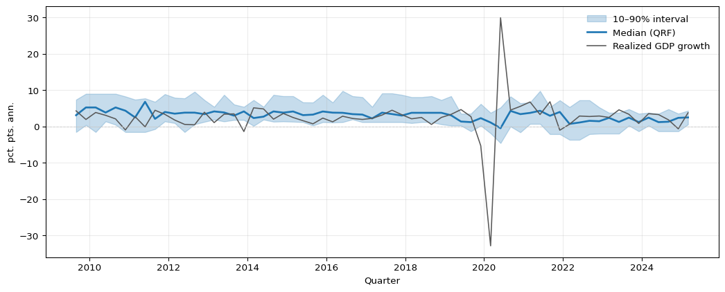
Figure 13.1 illustrates the method with the quarterly Federal Reserve Economic Data collection (FRED-QD) (McCracken and Ng 2020). The target is annualized gross domestic product (GDP) growth in quarter t+1, and the five predictors are dated quarter t.¹ The horizontal axis records the target quarter t+1. Look for both the changing width of the central 80% interval, formed by the estimated 10th and 90th conditional quantiles, and its behavior during the pandemic observations.

import numpy as np
import pandas as pd
import matplotlib.pyplot as plt
from sklearn.ensemble import RandomForestRegressor

raw = pd.read_csv("data/fred_qd_current.csv")
fred_qd = raw.iloc[2:].copy()
fred_qd["sasdate"] = pd.to_datetime(fred_qd["sasdate"])
for col in fred_qd.columns:
    if col != "sasdate":
        fred_qd[col] = pd.to_numeric(fred_qd[col], errors="coerce")
fred_qd = fred_qd.sort_values("sasdate").reset_index(drop=True)

gdp_growth  = 400 * np.log(fred_qd["GDPC1"]).diff()
inflation   = 400 * np.log(fred_qd["CPIAUCSL"]).diff()
term_spread = fred_qd["GS10"] - fred_qd["TB3MS"]
log_vix     = np.log(fred_qd["VIXCLSx"])

macro = pd.DataFrame({
    "target_date": fred_qd["sasdate"].shift(-1),
    "y":           gdp_growth.shift(-1),
    "gdp_lag1":    gdp_growth,
    "infl_lag1":   inflation,
    "spread_lag1": term_spread,
    "vix_lag1":    log_vix,
    "unrate_lag1": fred_qd["UNRATE"],
}).dropna()

feature_cols = ["gdp_lag1", "infl_lag1", "spread_lag1", "vix_lag1", "unrate_lag1"]
split = int(len(macro) * 0.75)
X_train = macro.iloc[:split][feature_cols].values
y_train = macro.iloc[:split]["y"].values
X_test  = macro.iloc[split:][feature_cols].values
y_test  = macro.iloc[split:]["y"].values
test_dates = macro.iloc[split:]["target_date"]

rf = RandomForestRegressor(
    n_estimators=200,
    max_features="sqrt",
    min_samples_leaf=5,
    random_state=42,
)
rf.fit(X_train, y_train)

# QRF: weighted empirical quantiles via leaf assignments
train_leaves = rf.apply(X_train)   # (n_train, n_trees)
test_leaves  = rf.apply(X_test)    # (n_test,  n_trees)
n_trees = train_leaves.shape[1]

# For each test point, accumulate normalized weights across trees
weights_matrix = np.zeros((len(X_test), len(X_train)))
for b in range(n_trees):
    same_leaf  = test_leaves[:, b:b+1] == train_leaves[np.newaxis, :, b]  # (n_test, n_train)
    leaf_sizes = same_leaf.sum(axis=1, keepdims=True).clip(min=1)
    weights_matrix += same_leaf / leaf_sizes
weights_matrix /= n_trees

# Weighted empirical quantiles
sorted_idx = np.argsort(y_train)
y_sorted   = y_train[sorted_idx]
q10, q50, q90 = [], [], []
for i in range(len(X_test)):
    cum_w = np.cumsum(weights_matrix[i, sorted_idx])
    cum_w /= cum_w[-1]
    q10.append(y_sorted[np.searchsorted(cum_w, 0.10)])
    q50.append(y_sorted[np.searchsorted(cum_w, 0.50)])
    q90.append(y_sorted[np.searchsorted(cum_w, 0.90)])

q10, q50, q90 = np.array(q10), np.array(q50), np.array(q90)

fig, ax = plt.subplots(figsize=(11, 4.5))
ax.fill_between(test_dates, q10, q90, alpha=0.25, color="C0", label="10–90% interval")
ax.plot(test_dates, q50,    color="C0",  linewidth=2,   label="Median (QRF)")
ax.plot(test_dates, y_test, color="0.35", linewidth=1.2, label="Realized GDP growth")
ax.axhline(0, color="0.8", linewidth=0.7, linestyle="--")
ax.set_xlabel("Quarter")
ax.set_ylabel("pct. pts. ann.")
ax.legend(frameon=False)
ax.grid(True, alpha=0.25)
plt.tight_layout()
plt.show()

Figure 13.1: QRF forecasts for one-step-ahead GDP growth (annualized log-difference of GDPC1) over the final 25% of FRED-QD quarters. The horizontal axis gives the target quarter. The blue band is the central 80% predictive interval spanning the estimated conditional 10th to 90th percentiles, the solid blue line is the estimated conditional median, and the gray line is realized GDP growth. Conditional quantiles use original-observation neighborhood weights from 200 trees with a minimum in-bag leaf size of five.

The interval width varies across the test period because the QRF neighborhood changes with the predictors. A homoskedastic fixed-shape location-scale model, such as a Gaussian location model with constant conditional variance, would instead impose a constant central-interval width around its conditional mean. Homoskedasticity alone would not do so if other shape parameters could vary with predictors. The estimated band is a central 80% predictive interval, not an automatic 80% coverage guarantee. Its marginal and conditional coverage are empirical calibration questions. A finite-sample guarantee would require an additional calibration method, such as those developed in the conformal-prediction chapter, under its own assumptions. The pandemic quarters expose the more immediate limitation. Realized growth reaches roughly -33 and then +30 annualized percent in 2020, while the forecast band remains far inside those values. By construction, \hat F(y \mid X=x) reweights outcomes observed in the training sample and therefore cannot place mass beyond their range. When the training neighborhood contains no comparable episode, changing the quantile level cannot recover the missing tail support.

This failure is the distributional counterpart of the extrapolation limit from the decision trees chapter: QRF interpolates among observed outcomes for the entire predictive distribution, not only for its mean. A parametric family with unbounded support, such as the NGBoost specification below, can represent outcomes beyond the training range, and an explicit extreme-value model can impose tail structure. Neither choice guarantees accurate pandemic-tail forecasts under a structural break; both still require time-aware validation and a defensible distributional specification.

13.7 NGBoost: Parametric Distributional Boosting

NGBoost takes a different route. Instead of estimating the conditional distribution nonparametrically from forest neighbors, it chooses a parametric family

Y\mid X=x \sim P_{\theta(x)}

and learns its parameters by boosting. The learner works in a coordinate vector \theta(x) on an unconstrained chart and maps those coordinates into valid distribution parameters. For a Gaussian distribution, for example, it can use \theta(x)=(\mu(x),\eta(x)) with \eta(x)=\log\sigma(x); a positive exponential rate can likewise be represented on the log scale.

To keep the formulas concrete, we use the negative log-likelihood (NLL), which is the logarithmic-score loss,

\ell(y;\theta)=-\log p_\theta(y).

This choice connects NGBoost to the distributional-network chapter and the predictive-distribution evaluation chapter: minimizing average NLL is the training analogue of optimizing the logarithmic score (see the Kullback–Leibler (KL) divergence connection). NGBoost can instead use another proper scoring rule, such as the continuous ranked probability score. In that case, the natural-gradient metric is derived from the local curvature of the divergence induced by that score and need not equal the Fisher information (Duan et al. 2020).

Standard Boosting vs NGBoost

Standard squared-error boosting learns one scalar prediction function, typically a conditional mean. NGBoost learns one or more functions that parameterize a full predictive distribution. The price of this richer output is that the researcher must choose a distributional family and respect its parameter constraints.

13.8 Natural Gradients and Fisher Scaling

NGBoost’s defining choice is the natural gradient. In an ordinary gradient step, parameters are updated using the Euclidean gradient of the loss. For distribution parameters, this can be poorly scaled: a one-unit change in a mean parameter and a one-unit change in a scale parameter need not have comparable effects on the predictive density. For the NLL case developed here, the relevant metric is Fisher information.

As in standard boosting, the path needs an initial prediction. NGBoost starts from the constant parameter vector that best fits the marginal training distribution,

\theta^{(0)} \in \arg\min_{\theta}\sum_{i=1}^N \ell(y_i;\theta),

so every training observation initially receives the same predictive distribution. This notation allows multiple minimizers; the discussion assumes that at least one finite interior solution exists. Boundary samples may instead require regularization, clipping, or rejection by the implementation. The boosted stages then let the coordinates, and hence the mapped distribution parameters, vary with x.

At iteration m, let

g_i^{(m)} = \left.\nabla_\theta \ell(y_i;\theta)\right|_{\theta=\theta^{(m-1)}(x_i)}

be the ordinary gradient for observation i. The Fisher information matrix—written \mathcal{I} to avoid a clash with the conditional CDF \hat F used earlier in this chapter—is

\mathcal{I}(\theta) = \mathbb{E}_{Y\sim P_\theta} \left[ \nabla_\theta \log p_\theta(Y) \nabla_\theta \log p_\theta(Y)^\top \right].

Assuming \mathcal{I}(\theta) is positive definite, the natural gradient rescales the ordinary gradient:

\tilde g_i^{(m)} = \mathcal{I}(\theta^{(m-1)}(x_i))^{-1}g_i^{(m)}.

Figure 13.2 makes the rescaling visible for a Gaussian negative log-likelihood parameterized by its mean \mu and log standard deviation \eta=\log\sigma. The contour lines are equal-loss sets for a five-observation sample. Both arrows start from the same parameter value and use the same nominal step size; they differ only in whether the loss gradient is used directly or premultiplied by inverse Fisher information.

import numpy as np
import matplotlib.pyplot as plt

y_demo = np.array([-2.0, -0.5, 0.0, 1.0, 2.0])
mu_grid = np.linspace(-2.5, 2.5, 260)
eta_grid = np.linspace(-1.0, 1.2, 240)
MU, ETA = np.meshgrid(mu_grid, eta_grid)
LOSS = ETA + 0.5 * np.mean(
    (y_demo[None, None, :] - MU[:, :, None]) ** 2
    * np.exp(-2.0 * ETA[:, :, None]),
    axis=2,
)
LOSS = LOSS - LOSS.min()

mu0, eta0 = -1.0, 0.4
mean_sq_resid = np.mean((y_demo - mu0) ** 2)
ordinary = np.array([
    np.exp(-2.0 * eta0) * (mu0 - y_demo.mean()),
    1.0 - np.exp(-2.0 * eta0) * mean_sq_resid,
])
fisher = np.diag([np.exp(-2.0 * eta0), 2.0])
natural = np.linalg.solve(fisher, ordinary)
step = 0.8

fig, ax = plt.subplots(figsize=(8.2, 4.8))
levels = [0.02, 0.05, 0.10, 0.20, 0.40, 0.80, 1.50, 2.50, 4.00]
contours = ax.contour(MU, ETA, LOSS, levels=levels, cmap="Greys")
ax.clabel(contours, inline=True, fontsize=8, fmt="%.2g")
ax.scatter([mu0], [eta0], color="black", s=45, zorder=4, label="Starting value")

for direction, color, label in [
    (ordinary, "C3", "Ordinary gradient"),
    (natural, "C0", "Natural gradient"),
]:
    delta = -step * direction
    ax.arrow(mu0, eta0, delta[0], delta[1], width=0.012,
             head_width=0.09, length_includes_head=True,
             color=color, alpha=0.9, label=label)

ax.set_xlabel(r"Mean parameter $\mu$")
ax.set_ylabel(r"Log standard deviation $\eta=\log\sigma$")
ax.set_title("Fisher scaling changes the descent direction")
ax.grid(True, alpha=0.18)
ax.legend(frameon=False)
plt.tight_layout()
plt.show()

Figure 13.2: Ordinary and natural-gradient descent directions for Gaussian negative log-likelihood in the parameterization (\mu,\eta), where \eta=\log\sigma. Contours show the sample-average loss above its minimum. Both arrows start at (\mu,\eta)=(-1,0.4) and use the same nominal step size.

In Figure 13.2, the ordinary direction reacts to the numerical coordinates themselves, whereas the natural direction measures a change relative to how much it moves the predictive distribution. At this starting point, Fisher scaling places relatively more weight on correcting the mean: the natural-gradient arrow moves farther horizontally and less vertically than the ordinary-gradient arrow. The figure is illustrative rather than a convergence comparison: line search and repeated boosted stages still determine the realized path.

The Bernoulli leaf update in the gradient-boosting chapter is a scalar instance of this Fisher-scaling idea. Its Newton denominator \sum_{i:\,x_i\in R_{jm}} p_{i,m-1}(1-p_{i,m-1}) is the Fisher curvature of the leaf’s log-odds parameter, so dividing the leaf score by that quantity is a one-parameter Fisher-scoring step. NGBoost extends that information scaling to a vector of distribution parameters and then approximates each component with a base learner.

This chapter uses a positive loss-gradient convention: NGBoost fits a weak learner \hat h_m(x) to \tilde g_i^{(m)} and subtracts the fitted direction. The gradient-boosting chapter instead defined pseudo-residuals as negative gradients and added the fitted tree; the two sign conventions describe the same descent step.

NGBoost chooses one stage-specific scale by a line search,

\rho^{(m)} = \arg\min_{\rho} \sum_{i=1}^N \ell\!\left(y_i;\theta^{(m-1)}(x_i)-\rho\,\hat h_m(x_i)\right),

and then applies the learning rate \nu\in(0,1]:

\theta^{(m)}(x) = \theta^{(m-1)}(x) - \nu\, \rho^{(m)}\, \hat h_m(x), \qquad m=1,\ldots,M.

This update is analogous to the stagewise descent of the previous chapter, now along a vector of distribution parameters. There is one important difference in the line search: \rho^{(m)} is a single scalar for the whole multi-parameter stage, whereas the exact loss-optimal \gamma_{jm}^{\star} in the gradient-boosting chapter is chosen separately for each leaf. The learning rate \nu, the number of iterations M, and the need for time-aware early stopping carry over. Fisher scaling makes the natural-gradient direction, viewed as an infinitesimal tangent vector, invariant to smooth one-to-one reparameterizations and prevents the numerical units of one parameter from dominating that direction (Duan et al. 2020). An ordinary finite coordinate update is an Euler step along this vector field and is only first-order invariant: applying separate finite steps in two parameterizations need not produce exactly corresponding parameter paths.

13.9 Parameterization and Update Choices

Distribution parameters often have constraints. A variance, standard deviation, rate, or scale parameter must be positive, and a probability must lie in (0,1). NGBoost implementations therefore usually predict unconstrained functions and transform them into valid distribution parameters.

Common constraint-preserving parameterizations include:

• predict \log \sigma(x) rather than \sigma(x)
• use a softplus transformation \zeta(z)=\log(1+e^{z}), which is smooth and strictly positive, to map a learned scalar score z(x) into a positive parameter \zeta(z(x))
• use a logistic transformation s(z)=1/(1+e^{-z}) for probabilities (written s here because \sigma already denotes a scale parameter in this chapter)

For a distribution with several parameters, standard NGBoost fits one base learner to each component of the natural gradient at every stage. For a Gaussian model, for example, one learner fits the mean component and another fits the log-scale component; together they form the vector \hat h_m(x). All components update simultaneously and share the stage scale \rho^{(m)}. A coordinate-wise cycle or a single multi-output learner would be a different algorithmic variant, not the standard NGBoost update.

13.10 QRF vs NGBoost

QRF and NGBoost both produce conditional predictive distributions, but in opposite ways: QRF is nonparametric (the conditional law is the weighted empirical distribution of training outcomes in a forest neighborhood), while NGBoost is parametric (the conditional law belongs to a chosen family, and boosting iteratively fits its parameters).

Method	Distributional object	Main advantage	Main limitation
QRF	Weighted empirical CDF from forest neighbors	Flexible shape and adaptive quantile intervals	Few local tail observations and no extrapolation beyond observed outcomes
NGBoost	Parametric distribution P_{\theta(x)}	Smooth distribution and proper-score-based training	Sensitive to distributional misspecification

In econometric work, the choice depends on the forecasting object. If the goal is flexible local quantiles with few parametric assumptions, QRF is natural. If the goal is a smooth parametric predictive distribution with proper-score-based training, NGBoost is more natural.

Both methods estimate uncertainty in the outcome Y\mid X=x. Neither fitted predictive distribution automatically quantifies sampling uncertainty about the estimated forest weights, trees, or parameter functions; confidence intervals for those estimated objects require separate inferential machinery.

13.11 Summary

Key Takeaways

1. Forest partitions define neighborhood weights through shared terminal leaves.
2. Quantile regression forests use these weights to estimate a conditional empirical CDF and its quantiles.
3. NGBoost fits parameters of a predictive distribution by minimizing a proper scoring rule.
4. Under log loss, natural gradients use inverse Fisher information to rescale parameter updates.

Common Pitfalls

• Reconstructing a bootstrap-forest mean requires resampling multiplicities, not just the original-observation QRF weights.
• Extreme conditional quantiles need enough relevant tail observations in the forest neighborhood.
• Enforce valid distributional parameters and choose support compatible with the outcome.
• A fitted predictive distribution does not automatically include uncertainty about the estimated model.

13.12 Exercises

Exercise 13.1: Quantile Regression Forest Prediction

At forecast origin t, you train a QRF with B=3 trees to forecast the next-period portfolio return Y_{t+1}, measured in basis points, from predictors X_t=x_{\text{new}} available at t. You collect the training observations that fall into the terminal leaf reached by x_{\text{new}} in each tree, identified by observation index i with outcome y_i:

• Tree 1 leaf: observations 3, 7, 9 with outcomes y_3=10, y_7=12, y_9=15
• Tree 2 leaf: observations 5, 6, 7 with outcomes y_5=8, y_6=11, y_7=12
• Tree 3 leaf: observations 7, 11, 14 with outcomes y_7=12, y_{11}=14, y_{14}=20

Note that observation 7 is a neighbor in all three trees, while the other six observations appear in exactly one leaf each.

Questions:

1. Pool and sort the nine neighbor appearances. Then use the weight representation w_i(x_{\text{new}}) = \frac{1}{B}\sum_{b=1}^B \frac{\mathbf{1}\{x_i \in L_b(x_{\text{new}})\}}{N_b(x_{\text{new}})}, to derive each observation’s weight and the resulting probability mass on each distinct outcome value. Construct the weighted empirical CDF \hat F(y \mid X=x_{\text{new}}) and use \widehat{q}_{\alpha}(x_{\text{new}})=\inf\{y:\hat F(y\mid X=x_{\text{new}})\ge \alpha\} to compute the predicted conditional median and conditional 25th percentile.
2. Explain why the repeated appearance of observation 7 should not be removed, and distinguish it from a case in which three different observations happen to have the same outcome value.
3. Across a long out-of-sample evaluation, a dependence-robust coverage test rejects the null that realized returns fall below the estimated 10% quantile with probability 10%; the observed violation rate is higher. State what this establishes about 10% quantile calibration, give two distinct misspecification mechanisms that the test does not distinguish, and name one additional diagnostic that would help separate them.
4. Use the weighted empirical CDF to show that every fitted QRF quantile lies between the smallest and largest training outcome with positive weight at x_{\text{new}}. State the implication for forecasting an unprecedented tail realization below all positively weighted outcomes.

Exam level. Part 1 connects pooled neighbors to forest weights and weighted empirical quantiles, Part 2 checks the neighborhood interpretation, Part 3 adds a tail-calibration diagnostic, and Part 4 establishes the support limitation.

Hint for Part 3

Separate what the coverage result determines from what it leaves open. Sketch two forecast distributions—one shifted, one too narrow—that would both produce the same excess violation rate.

Solution

Part 1: Neighbor weights, CDF, and quantiles

Pooling gives

\{10,12,15,8,11,12,12,14,20\}.

Sorted, this is

\{8,10,11,12,12,12,14,15,20\},

with nine total neighbor appearances.

Each tree receives weight 1/3, and that weight is divided equally among its three leaf neighbors. One appearance in one tree therefore contributes

\frac{1}{3}\cdot \frac{1}{3}=\frac{1}{9}.

Observation 7 appears three times and receives weight 1/3; each other observation appears once and receives weight 1/9. Aggregating observations by outcome value gives

\begin{aligned} 8 &:\frac{1}{9}, \\ 10 &:\frac{1}{9}, \\ 11 &:\frac{1}{9}, \\ 12 &:\frac{3}{9}=\frac{1}{3}, \\ 14 &:\frac{1}{9}, \\ 15 &:\frac{1}{9}, \\ 20 &:\frac{1}{9}. \end{aligned}

Thus the outcome value 12, carried here by observation 7, receives the largest probability mass.

The weighted empirical CDF places mass on the sorted distinct outcomes as follows:

y	Weight	Cumulative weight
8	1/9	1/9
10	1/9	2/9
11	1/9	3/9
12	1/3	6/9
14	1/9	7/9
15	1/9	8/9
20	1/9	1

For the median, we need the first value where cumulative weight reaches at least 0.5. That happens at y=12, so

\widehat q_{0.5}(x_{\text{new}})=12.

For the 25th percentile, we need the first value where cumulative weight reaches at least 0.25. Since

\frac{2}{9}<0.25\le \frac{3}{9},

the conditional 25th percentile is

\widehat q_{0.25}(x_{\text{new}})=11.

Part 2: Repeated observations and repeated values

Duplicates reflect forest weights. Here observation 7 is a neighbor in all three trees, so it receives weight 3 \times \tfrac{1}{3}\cdot\tfrac{1}{3} = \tfrac{1}{3}, three times the weight of any observation that appears in a single leaf. That is the forest’s statement that observation 7 is more local to x_{\text{new}} than the others, and discarding the repetition would discard exactly that information.

The identification matters: what carries the weight is the repeated observation, not the repeated value. Had three distinct observations happened to share the outcome 12, the weighted CDF would look identical at that point, but the interpretation would be different—three separate neighbors agreeing on an outcome, rather than one neighbor counted three times. In practice one works with observation indices, precisely so the two cases can be told apart.

Part 3: Tail calibration

The determinate conclusion is about calibration, not mechanism: the rejection and the violation rate above 10% show that the forecasts fail unconditional 10% quantile calibration and understate downside risk in frequency terms. The coverage test does not establish that the estimated quantile is above the true conditional quantile at every date, or even on average under a particular numerical measure of distance.

The violation count does not identify why calibration fails. A systematically optimistic center with otherwise adequate dispersion and a well-centered forecast with too little dispersion can both produce excess violations; so can a left tail that is too thin or failures concentrated in stressed periods. Median forecast errors help diagnose a location shift, calibration at several quantile levels helps distinguish a general dispersion problem from a local tail problem, and the time sequence of violations reveals whether failures cluster.

Part 4: Predictive support

Let y_{\mathrm{min}}(x) and y_{\mathrm{max}}(x) be the smallest and largest training outcomes with w_i(x)>0. The weighted CDF is zero below y_{\mathrm{min}}(x) and equals one at and above y_{\mathrm{max}}(x). Its generalized inverse therefore satisfies

y_{\mathrm{min}}(x)\leq \widehat q_\alpha(x)\leq y_{\mathrm{max}}(x) \qquad\text{for every }\alpha\in(0,1).

At x_{\text{new}}, this interval is [8,20]. Lowering the quantile level can move the forecast only among positively weighted training outcomes; it cannot assign a fitted quantile below 8 or recover a genuinely unprecedented left-tail event.

Exercise 13.2: NGBoost with Exponential Likelihood

Assume we model a positive target variable Y with a conditional exponential distribution:

Y \mid X=x \sim \text{Exp}(\lambda(x)), \qquad f(y;\lambda)=\lambda e^{-\lambda y} \quad \text{for } y\ge 0, \qquad \lambda>0.

NGBoost can be used to learn the rate parameter function \lambda(x).

Questions:

1. Contrast NGBoost with standard gradient boosting under mean squared error (MSE) and with QRF along three dimensions: the prediction produced, the distributional assumption, and the object fitted at each boosting or forest step.
2. Derive the per-observation NLL \ell(y;\lambda) and its ordinary gradient \partial \ell/\partial \lambda. Given the Fisher information \mathcal{I}_{\lambda\lambda}=1/\lambda^2, derive the natural gradient \tilde g_\lambda=\mathcal{I}_{\lambda\lambda}^{-1}\partial \ell/\partial \lambda.
3. For \lambda=0.4 and y=3, compute the ordinary and natural gradients. For a single-observation descent step with a positive step size small enough to keep \lambda>0, state whether \lambda and the implied conditional mean 1/\lambda move up or down.
4. Let \theta(x)=\log \lambda(x), so \lambda=e^\theta. Derive \partial \ell/\partial \theta, \mathcal{I}_{\theta\theta}, and the natural gradient in the \theta parameterization. Show that mapping this infinitesimal direction back to the \lambda scale gives the natural-gradient direction from Part 2.
5. Explain why the agreement of the infinitesimal directions in Part 4 does not imply that ordinary finite Euler updates in the two coordinates generate exactly matching parameter sequences. Then explain how the log-rate parameterization enforces the constraint \lambda>0.
6. For an exponential distribution, both the conditional mean and the conditional standard deviation, written \operatorname{SD}(Y\mid X=x), equal 1/\lambda(x). Suppose that, at a particular predictor value x, the conditional mean is 2 and the conditional standard deviation is 4. Show that no value of \lambda(x) matches both features, and explain why allowing a flexible function \lambda(x) cannot remove this distributional misspecification.

Exam level. The exercise connects model comparison, likelihood calculation, reparameterization, finite-step interpretation, and a testable restriction of the exponential family.

Hint for Part 4

Use the chain rule and the information transformation:

\frac{\partial \ell}{\partial \theta} = \frac{\partial \ell}{\partial \lambda} \frac{\partial \lambda}{\partial \theta}, \qquad \mathcal I_{\theta\theta} = \mathcal I_{\lambda\lambda} \left(\frac{\partial \lambda}{\partial \theta}\right)^2.

Solution

Part 1: Conceptual comparison

Standard gradient boosting under MSE produces a scalar point prediction, typically an estimate of the conditional mean. It imposes no complete predictive distribution and fits each new tree to residuals, which are the negative squared-error gradients. QRF produces a weighted empirical conditional distribution without choosing a parametric family; its weights come from how often observations share forest leaves with the forecast point. NGBoost produces a parametric conditional distribution and fits one sequence of base learners per distribution parameter to natural-gradient targets from a proper scoring rule.

Part 2: NLL and ordinary gradient

The negative log-likelihood is

\ell(y;\lambda) = -\log(\lambda e^{-\lambda y}) = -\log\lambda+\lambda y.

Therefore

\frac{\partial \ell}{\partial \lambda} = -\frac{1}{\lambda}+y.

Since \mathcal I_{\lambda\lambda}=1/\lambda^2, its inverse is \lambda^2. Hence

\tilde g_\lambda = \lambda^2\left(-\frac{1}{\lambda}+y\right) = -\lambda+\lambda^2y = \lambda(\lambda y-1).

Part 3: Numeric calculation and update direction

With \lambda=0.4 and y=3,

\frac{\partial \ell}{\partial \lambda} = -\frac{1}{0.4}+3 = -2.5+3 = 0.5.

The natural gradient is

\tilde g_\lambda = -0.4+(0.4)^2\cdot 3 = -0.4+0.48 = 0.08.

Both gradients are positive. Because the update subtracts the fitted positive gradient direction, a sufficiently small single-observation descent step decreases \lambda. The exponential conditional mean 1/\lambda therefore increases from its current value 1/0.4=2.5, moving toward the observed value y=3.

Part 4: Log-rate parameterization and invariance

Because \lambda=e^\theta,

\frac{\partial \lambda}{\partial \theta}=e^\theta=\lambda.

Thus

\frac{\partial \ell}{\partial \theta} = \left(-\frac{1}{\lambda}+y\right)\lambda = -1+y e^\theta.

The Fisher information transforms as

\mathcal I_{\theta\theta} = \mathcal I_{\lambda\lambda} \left(\frac{\partial \lambda}{\partial \theta}\right)^2 = \frac{1}{\lambda^2}\lambda^2 =1.

The natural gradient on the log-rate scale is therefore

\tilde g_\theta = \mathcal I_{\theta\theta}^{-1} \frac{\partial\ell}{\partial\theta} = \lambda y-1.

For a small change, d\lambda=(\partial\lambda/\partial\theta)d\theta=\lambda\,d\theta. Mapping the natural-gradient direction back to the rate scale gives

\lambda\tilde g_\theta = \lambda(\lambda y-1) = \tilde g_\lambda,

which is the direction obtained in Part 2. This agreement establishes the coordinate transformation of the infinitesimal natural-gradient direction.

Part 5: Finite coordinate updates and the positivity constraint

The agreement in Part 4 concerns an infinitesimal direction. After a finite log-rate step \Delta\theta, the exact mapped change is \lambda(e^{\Delta\theta}-1), which equals \lambda\Delta\theta only to first order. Ordinary finite Euler updates carried out separately in the two coordinates can therefore generate different parameter sequences.

The log-rate parameterization also turns the constrained rate \lambda>0 into an unconstrained parameter \theta\in\mathbb{R}. Any finite value of \theta maps to \lambda=e^\theta>0, so every update produces a valid rate.

Part 6: Exponential-family misspecification

Matching the conditional mean 2 requires

\frac{1}{\lambda(x)}=2, \qquad\text{so}\qquad \lambda(x)=\frac{1}{2}.

At that rate, the exponential model also imposes a conditional standard deviation of 2, not 4. Matching the conditional standard deviation instead requires \lambda(x)=1/4, which imposes a conditional mean of 4, not 2. No rate matches both moments.

Letting \lambda(x) be an arbitrarily flexible function changes the common level 1/\lambda(x) across predictor values, but it never breaks the exponential restriction that the conditional mean equals the conditional standard deviation at each x. Addressing this failure requires a richer distributional family with separate location and scale behavior, not merely more flexible trees for the same one-parameter family.

13.13 References

Athey, Susan, Julie Tibshirani, and Stefan Wager. 2019. “Generalized Random Forests.” Annals of Statistics 47 (2): 1148–78. https://doi.org/10.1214/18-AOS1709.

Duan, Tony, Anand Avati, Daisy Yi Ding, Khanh K. Thai, Sanjay Basu, Andrew Y. Ng, and Alejandro Schuler. 2020. “NGBoost: Natural Gradient Boosting for Probabilistic Prediction.” In Proceedings of the 37th International Conference on Machine Learning, 119:2690–700. Proceedings of Machine Learning Research.

McCracken, Michael W., and Serena Ng. 2020. “FRED-QD: A Quarterly Database for Macroeconomic Research.” Working Paper 26872. National Bureau of Economic Research. https://doi.org/10.3386/w26872.

Meinshausen, Nicolai. 2006. “Quantile Regression Forests.” Journal of Machine Learning Research 7: 983–99.

Wager, Stefan, and Susan Athey. 2018. “Estimation and Inference of Heterogeneous Treatment Effects Using Random Forests.” Journal of the American Statistical Association 113 (523): 1228–42. https://doi.org/10.1080/01621459.2017.1319839.

Footnotes

1. This is a pedagogical final-vintage FRED-QD example. The forest settings are illustrative rather than test-set-tuned. A full real-time GDP forecasting evaluation would choose them inside a time-aware training/validation design and account for release calendars and data revisions.