Under active development. A stable version is expected in November 2026. Feedback is welcome by email or via GitHub issues.
5 Feed-Forward Neural Networks
5.1 Overview
Feed-forward neural networks are best understood as flexible nonlinear regression models. In classical econometrics, we often begin with a parametric specification such as a linear model, a polynomial expansion, or a spline basis. A feed-forward neural network keeps the same basic goal, estimating a conditional mean or conditional class probability, but replaces hand-crafted basis functions by a learned composition of affine transformations and nonlinear activation functions.
For econometricians, the main attraction is not mystery but flexibility. When the relationship between \(Y\) and \(\mathbf{X}\) is nonlinear, high-dimensional, or shaped by complicated interactions, a neural network offers a way to approximate that relationship without fully specifying it in advance. This is useful in applications such as the nonlinear asset-pricing setting studied by Gu, Kelly, and Xiu (2020) and in other prediction problems with large information sets:
Asset pricing: mapping many firm characteristics into expected returns
Macroeconomic forecasting: combining large predictor sets, survey variables, or text-based indicators
Household or firm behavior: approximating nonlinear Engel curves, production relationships, or treatment-response surfaces
Throughout this chapter, the econometric interpretation remains central: a feed-forward network is a flexible estimator of a regression function, but its flexibility comes with non-convex optimization, many tuning choices, and a higher risk of overfitting.
5.2 Roadmap
We begin with the simplest building block, the perceptron, and then build up the architecture of feed-forward networks as flexible nonlinear basis expansions.
We then discuss activation functions and the universal approximation theorem to clarify why nonlinear layers matter.
Next, we connect neural-network estimation to loss minimization, maximum likelihood, gradient descent, and backpropagation.
We then discuss non-convexity, econometric interpretation, and practical training decisions.
The chapter closes with applications, a chapter summary, common pitfalls, and exercises.
5.3 Basic Architecture
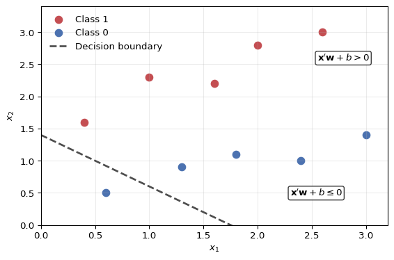
A neural network is a composition of affine maps and nonlinear activations, organized in layers with weights that adjust during learning. The cleanest entry point is a single unit: the perceptron takes predictors \(\mathbf{x}\), forms the affine score \(\mathbf{x}'\mathbf{w}+b\), and applies an activation function \(g\):
\[
\hat y = g(\mathbf{x}'\mathbf{w}+b).
\]
We call such a single unit a neuron (the terms unit and neuron are used interchangeably). If \(g\) is the identity, this is a linear regression. If \(g\) is a sigmoid, the same affine score becomes a probability-like output for binary classification. The perceptron is a single-index model with a nonlinear link function — a special case of the generalized linear model (GLM) family. Depth (composing multiple such layers) is what distinguishes a neural network from this baseline.
Figure 5.1: A single perceptron classifies observations by applying an activation to an affine score. The dashed line is the zero-score decision boundary \(x_2 = 1.4 - 0.8x_1\). Points on opposite sides of the boundary receive different classifications.
The only nonlinear element in Figure 5.1 is the activation or threshold applied after the affine score. A feed-forward network simply stacks many such units, so that the outputs of one layer become regressors for the next layer. That is why neural networks can be understood as learned basis expansions rather than as a fundamentally alien model class. In a polynomial or spline regression, the transformed regressors are chosen before estimation; in a neural network, the hidden activations \(a_j^{(l)}\) (the activation of unit \(j\) in layer \(l\), defined formally below) are themselves learned from the data.
A feed-forward neural network with \(L\) layers (that is, \(L-1\) hidden layers followed by an output layer indexed \(L\)) can be written as a composition
The layers play distinct roles: the input layer holds the predictors \(\mathbf{x}\), the hidden layers compute intermediate activations, and the output layer produces the prediction \(\hat{\mathbf y}\). Concretely, each layer \(l\) computes:
\(\mathbf{a}^{(l)}\) is the output of layer \(l\) (with \(\mathbf{a}^{(0)} = \mathbf{x}\))
\(\mathbf{W}^{(l)}\) is the weight matrix for layer \(l\), with dimensions \(H^{(l)} \times H^{(l-1)}\); the entry \(W_{ij}^{(l)}\) connects neuron \(j\) in layer \(l-1\) to neuron \(i\) in layer \(l\), where \(H^{(l)}\) is the number of units (width) of layer \(l\), with \(H^{(0)}=p\) the input dimension
\(\mathbf{b}^{(l)}\) is the bias vector for layer \(l\)
\(g^{(l)}\) is the activation function for layer \(l\), applied per vector entry
\(\boldsymbol{\theta}\) represents all hidden-layer and output-layer parameters
Moreover, we define the following quantity; the pre-activation value in layer \(l\): \(\mathbf{z}^{(l)} = \mathbf{W}^{(l)}\mathbf{a}^{(l-1)} + \mathbf{b}^{(l)}\).
Example of a Feed-forward Neural Network Architecture With Two Hidden Layers
The diagram in Figure 5.1 shows one unit. The architecture diagram above shows what changes in a multilayer network: instead of specifying a basis expansion by hand, we let the model learn many intermediate transformed regressors \(a_j^{(l)}\) and then combine them again in later layers.
Single Hidden Layer Networks
For the exercises, we’ll focus on single hidden layer networks, which have the form:
\(w_j^{(1)}, b_j^{(1)}\) are the input-to-hidden weights and biases
\(w_j^{(2)}, b^{(2)}\) are the hidden-to-output weights and bias
\(g(\cdot)\) is the activation function
Why Width and Depth Matter Quantitatively. A useful discipline is to count parameters before discussing “big” or “small” networks. If the input dimension is \(p\), a single-hidden-layer network with \(H\) hidden units and one scalar output contains
\[
(p+1)H + (H+1) = H(p+2)+1
\]
parameters: \(pH\) input-to-hidden weights, \(H\) hidden biases, \(H\) hidden-to-output weights, and one output bias. Even moderate changes in width can therefore increase estimation variance quickly when \(p\) is already large.
More generally, a fully connected network with hidden widths \(H^{(1)}, \dots, H^{(L)}\) and one scalar output has
parameters. This is one reason why validation discipline matters so much in econometric applications: architecture choice is itself a high-dimensional tuning problem, not just a cosmetic modeling choice.
Question for Reflection
Suppose a macro forecasting problem has \(p=40\) predictors and you compare one hidden layer with \(H=10\) against one hidden layer with \(H=100\). How many parameters does each network have, and what does that imply for overfitting risk?
Suggested Answer
With one scalar output, the count is \(H(p+2)+1\). For \(H=10\), this gives \(10(42)+1=421\) parameters. For \(H=100\), it gives \(100(42)+1=4201\) parameters. The larger network is much more flexible, but it also has roughly ten times as many free parameters, so it can fit idiosyncratic sample noise much more easily unless the sample is large and validation supports the extra complexity.
Use case: Hidden layers when zero-centered outputs are desired; historically often preferred to sigmoid in hidden layers because optimization tends to be more stable
Rectified Linear Unit (ReLU): \(\text{ReLU}(z) = \max(0, z)\)
Range: \([0, \infty)\)
Derivative: \(\text{ReLU}'(z) = \begin{cases} 1 & \text{if } z > 0 \\ 0 & \text{if } z \leq 0 \end{cases}\)
Use case: Hidden layers in deep networks; output layer for non-negative regression when smoothness at zero is not required (otherwise use softplus)
Softplus: \(\text{Softplus}(z) = \ln(1 + e^z)\)
Range: \((0, \infty)\)
Smooth approximation to ReLU
Use case: Output layer for non-negative continuous outcomes
Range: \((0, 1)\) with \(\sum_{i=1}^K \text{Softmax}(\mathbf{z})_i = 1\)
Derivative: \(\frac{\partial \text{Softmax}(\mathbf{z})_i}{\partial z_j} = \text{Softmax}(\mathbf{z})_i(\delta_{ij} - \text{Softmax}(\mathbf{z})_j)\), where \(\delta_{ij}=1\) if \(i=j\) and \(0\) otherwise (the Kronecker delta), which is distinct from the backprop error signal \(\delta_i^{(l)}\) introduced later
Use case: Output layer for multi-class classification
Linear/Identity: \(\text{Identity}(z) = z\)
Range: \((-\infty, \infty)\)
Use case: Output layer for regression problems
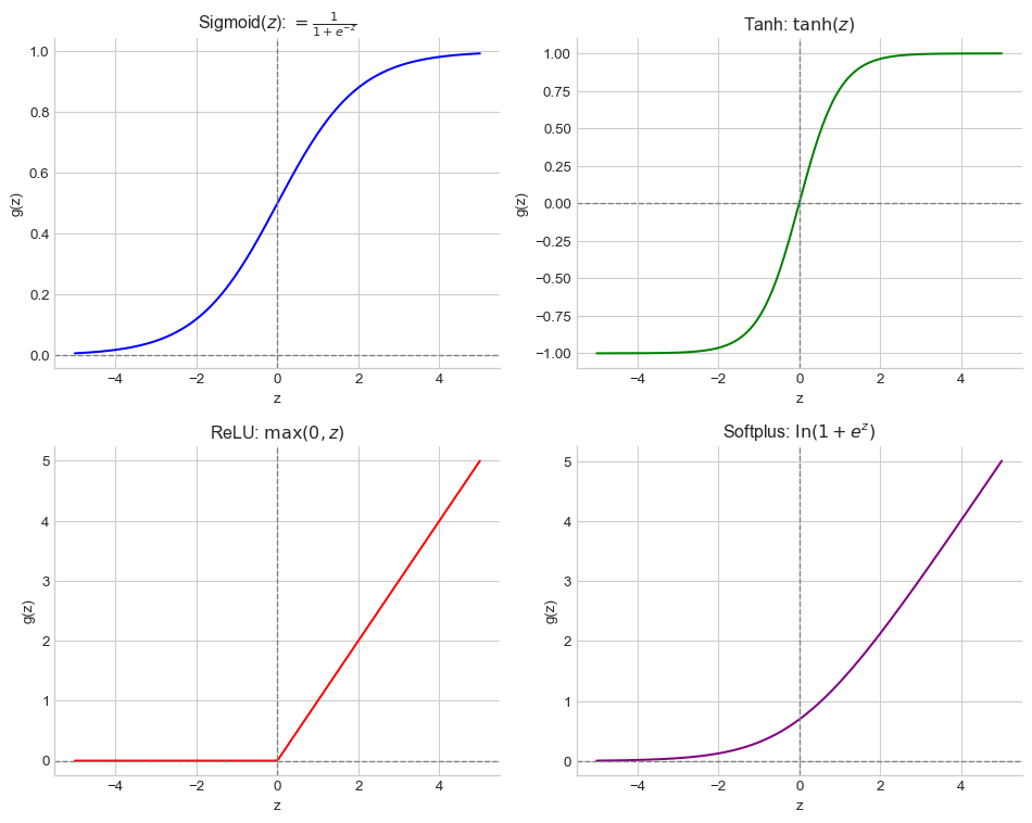
Figure 5.2 shows the four most common activation functions.
Figure 5.2: The four most common activation functions — Sigmoid, Tanh, ReLU, and Softplus — plotted against the pre-activation input \(z\) (x-axis) and their output \(g(z)\) (y-axis), arranged in a 2×2 grid. Dashed reference lines mark zero on both axes.
Each function provides a different kind of non-linearity, from the bounded “S-shape” of the sigmoid and tanh to the unbounded, one-sided linearity of ReLU and its smooth counterpart, Softplus.
Non-Differentiability and Backpropagation
ReLU is not differentiable at \(z=0\). In practice, software chooses a convention for the derivative at the kink, usually 0 or another subgradient; see the discussion of ReLU and other activation functions in Goodfellow, Bengio, and Courville (2016). This convention rarely matters for continuous inputs because hitting exactly \(z=0\) has probability zero under small perturbations, but it is worth remembering that backpropagation through piecewise-linear activations uses these derivative conventions at kink points.
Consider Tanh: For RNNs or when zero-centered outputs desired (sometimes better numerically)
For Output Layers (determined by problem type):
Regression problems (unbounded): Linear activation
Regression (positive): Softplus
Binary classification: Sigmoid for probability interpretation
Multi-class Classification: Softmax
Why Activation Functions Matter: Without activation functions, a deep neural network collapses into a single linear model. With two layers of weight matrices \(W_1\) and \(W_2\) and zero biases for exposition, the output of a linear-activation network is again a matrix times the input:
Using the output-layer guidelines above, what activation is natural for a positive regression outcome such as firm sales or volatility? If the loss is MSE, what target is the network learning?
Suggested Answer
Using the tools introduced in this chapter, a natural raw-scale choice is a softplus output with mean squared error. The softplus activation respects the non-negative support of the outcome, while MSE targets a conditional mean. The important econometric point is that the activation restricts the support of the prediction, while the loss determines the statistical target. MSE is about conditional-mean prediction, not the full conditional distribution.
Universal Approximation Theorem
Theorem (Cybenko 1989; Hornik 1991): Suppose \(g\) is a nonconstant, bounded, continuous activation function, such as a sigmoid. For any continuous function \(f\) on a compact (i.e., bounded and closed) set \(K\) and any \(\varepsilon > 0\), there exist a positive integer \(H\) and parameters \(\{w_j^{(1)}, b_j^{(1)}, w_j^{(2)}\}_{j=1}^{H}\) and \(b^{(2)}\) such that the function
The theorem is an existence result: it says a suitable width \(H\) exists, but does not tell us how to pick \(H\) or how to find the weights.
The notation here matches the single-hidden-layer representation introduced above. The same result extends from scalar \(x\) to vector-valued \(\mathbf{x} \in \mathbb{R}^k\).
The activation condition matters. The Cybenko-Hornik statement quoted here is the classical bounded-activation theorem, with sigmoids as the leading example. Modern networks often use ReLU, which is unbounded and therefore not covered by this version of the theorem. The classical extension that does cover ReLU is Leshno et al. (1993), who show that a single-hidden-layer network is a universal approximator on compact sets if and only if the activation is not a polynomial; this class includes ReLU and its variants. The practical lesson is the same – width can approximate rich nonlinear functions on compact domains – but the theorem being invoked is not literally the same theorem for every activation family.
Practical Implications
The theorem provides existence, not construction. It says that some width \(H\) suffices, but it does not say how to choose \(H\), how to find the weights, or how easy the resulting optimization will be. The width required in practice can be very large, and the underlying non-convex optimization remains hard whether or not the approximation theorem applies.
Loss Functions and Optimization
Mean Squared Error Loss (Regression)
For regression problems, we typically use the mean squared error:
The factor of \(\frac{1}{2}\) is sometimes included for convenience when taking derivatives. We can employ other loss functions as well to which we come back when discussing distributional networks.
Cross-Entropy Loss (Classification)
For binary classification problems, we typically use the cross-entropy (log-likelihood) loss. Let \(s_i=f(x_i;\boldsymbol{\theta})\) denote the network’s final real-valued score before the output sigmoid. If \(y_i \in \{0, 1\}\) are the true class labels and \(\hat{p}_i=\sigma(s_i)\) are the predicted probabilities, where \(\sigma\) is the sigmoid function defined above, then
where \(y_{ik}\) is the one-hot encoded true label (for a definition see callout box below) and \(\hat{p}_{ik} = \frac{\exp(f_k(x_i; \boldsymbol{\theta}))}{\sum_{j=1}^K \exp(f_j(x_i; \boldsymbol{\theta}))}\) is the softmax probability for class \(k\).
Definition: One-hot Encoding
One-hot encoding is a process of converting categorical variables into a binary vector representation. For a categorical variable with \(K\) possible classes, each observation is represented by a vector of length \(K\). This vector contains a single ‘1’ in the position corresponding to the observation’s class and ’0’s in all other positions.
Example: Suppose we are classifying economic regimes into three categories: “Recession”, “Normal”, and “Boom”. - A data point belonging to “Recession” would be encoded as [1, 0, 0]. - A data point belonging to “Normal” would be encoded as [0, 1, 0]. - A data point belonging to “Boom” would be encoded as [0, 0, 1].
This representation is useful because it allows machine learning models, which operate on numerical inputs, to handle categorical data without implying an ordinal relationship between the categories (e.g., that “Boom” is ‘greater’ than “Recession”).
Connection to Information Theory
The cross-entropy loss is not just a convenient formula — it has a direct information-theoretic foundation. Recall from the Information Theory chapter that minimizing cross-entropy between the empirical data distribution and the model is equivalent to maximum likelihood estimation, which in turn minimizes the KL divergence between the two distributions. When we train a neural network with cross-entropy loss, we are implicitly finding the parameters \(\boldsymbol{\theta}\) whose predicted class probabilities are closest (in KL divergence) to the true conditional class distribution.
Question for Reflection
Why is the cross-entropy loss for binary classification a special case of the categorical cross-entropy loss with \(K = 2\)?
Suggested Answer
With \(K = 2\), the one-hot outcome vector has two entries, for example \((y_i, 1-y_i)\), and the softmax probability vector is \((p_i, 1-p_i)\). Plugging these into the categorical cross-entropy loss
which is exactly the binary cross-entropy loss. So the binary case is not a different principle; it is the two-class version of the general categorical formula.
Gradient Descent Optimization
Unlike OLS with its convex quadratic objective, neural networks are typically trained by minimizing non-convex loss functions using gradient-based methods. Non-convexity raises several difficulties that gradient-based training must cope with:
Local minima: points where gradients are zero but the solution is not globally optimal
Saddle points: common in high dimensions, where the gradient is zero but the point is neither a minimum nor a maximum
Plateaus: flat regions where gradients are close to zero, slowing learning
We sketch the basic gradient-descent step here; the optimization chapter gives a more detailed discussion.
The gradient descent update rule with learning rate \(\eta\) is:
The gradient descent algorithm iteratively moves in the direction of steepest descent (negative gradient) to minimize the loss function. The learning rate \(\eta\) controls the step size, and convergence is typically checked by monitoring the gradient magnitude or loss change.
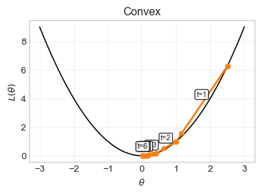
Convex function (left): Any initialization converges to the unique global minimum; step sizes naturally shrink as the gradient norm decreases.
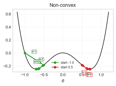
Non-convex function (right): Different initializations can fall into different local minima; one of these can be worse than the global minimum.
Neural networks: Their highly non-convex loss landscapes make optimization sensitive to initialization and learning rate choices.
Gradient Descent in The Simplest of Networks Consider a simple single hidden layer network with one neuron of the following form:
\[f(x; \boldsymbol{\theta}) = w_2 g(w_1 x + b_1) + b_2\]
Note that we deviate from indicating the layer by superscripts because in one of the exercises we use the superscript to denote a gradient descent update for this simple network.
For a sigmoid hidden activation, \(g'(z)=g(z)(1-g(z))\). The gradients of this loss for \(n\) data points \((x_i, y_i)\) are computed using the chain rule:
Let \(z = w_1 x + b_1\), \(a = g(z)\), and \(\hat{y} = w_2 a + b_2\).
For observation \(i\) with residual \(r_i = y_i - \hat{y}_i\):
The gradient descent procedure for a neural network can be visualized as follows:
flowchart TD
    %% Starting point
    START["θ⁽⁰⁾ (Initial Parameters)"] --> FORWARD["Forward Pass: Compute f(x; θ⁽ᵗ⁾)"]

    %% Forward computation
    FORWARD --> LOSS["Compute Loss L(θ⁽ᵗ⁾)"]

    %% Gradient computation
    LOSS --> GRAD["Compute Gradients ∇L(θ⁽ᵗ⁾)"]

    %% Parameter update
    GRAD --> UPDATE["Update: θ⁽ᵗ⁺¹⁾ = θ⁽ᵗ⁾ - η∇L(θ⁽ᵗ⁾)"]

    %% Convergence check
    UPDATE --> CHECK{"Converged?<br/>|∇L(θ⁽ᵗ⁺¹⁾)| < ε"}
    CHECK -->|No| FORWARD
    CHECK -->|Yes| OPTIMAL["θ* (Optimal Parameters)"]

    %% Styling
    classDef startend fill:#e8f5e8,stroke:#333,stroke-width:2px
    classDef process fill:#e1f5fe,stroke:#333,stroke-width:2px
    classDef decision fill:#fff3e0,stroke:#333,stroke-width:2px
    classDef update fill:#f3e5f5,stroke:#333,stroke-width:2px

    class START,OPTIMAL startend
    class FORWARD,LOSS,GRAD process
    class CHECK decision
    class UPDATE update
Figure 5.4: Flowchart of the gradient descent algorithm. Rectangular nodes represent computation steps (forward pass, loss evaluation, gradient computation, parameter update) and the diamond node is the convergence check. The loop continues until the gradient norm falls below a threshold \(\varepsilon\), at which point the current parameters are returned as the solution.
Backpropagation Algorithm for Multi-Layer Neural Networks
We now examine how the chain rule can be used to compute the gradient w.r.t. all parameters in an efficient way even if we look at a wide multi-layer network with entities defined as in Section 5.3. The algorithm, popularized by Rumelhart, Hinton, and Williams (1986), computes the gradients of the loss with respect to every weight and bias in a single backward sweep that reuses intermediate quantities from the forward pass. For gradient descent updates, we are interested in deriving
\[\frac{\partial L}{\partial W_{ij}^{(l)}} \text{ and } \frac{\partial L}{\partial b_i^{(l)}}\]
for all neurons \(i\) in all layers \(l\) and all neurons \(j\) in layer \(l-1\).
Error Signal Definition We define the following key quantity for each neuron \(i\) in layer \(l\):
This represents how much the loss would change if we perturb the pre-activation value of neuron \(i\) in layer \(l\). If we know this quantity at all nodes in our network, then we can easily compute all gradients because for each weight\(W_{ij}^{(l)}\) (connecting neuron \(j\) in layer \(l-1\) to neuron \(i\) in layer \(l\)):
For the output layer\(L\), \(\delta_i^{(L)}\) can be easily calculated as the first term is the derivative of a loss function like the MSE and the derivatives of the common activation functions (i.e., \(g'\)) are typically simple to compute:
Notice that we end up with \(W_{ji}^{(l+1)}\) (not \(W_{ij}^{(l+1)}\)), which connects neuron \(i\) (from layer \(l\)) to neuron \(j\) (in layer \(l+1\)).
Combining step 1 and 2, gives us the following insight: Backpropagation is also called Error Propagation because each neuron’s error signal \(\delta_i^{(l)}\) is computed as a weighted sum of error signals from the next layer. The recursion has a clean temporal reading: each backward step consumes the vector \(\boldsymbol{\delta}^{(l+1)}\) that was finished at the previous step and produces\(\boldsymbol{\delta}^{(l)}\) for the next step, with only one quantity — the local gate \(g'^{(l)}(\mathbf{z}^{(l)})\) — computed fresh at layer \(l\):
\[\delta_i^{(l)} = \underbrace{\left(\sum_{j=1}^{H_{l+1}} W_{ji}^{(l+1)} \delta_j^{(l+1)}\right)}_{\text{reused from step } l+1} \times \underbrace{g'^{(l)}(z_i^{(l)})}_{\text{computed fresh at layer } l}\]
Matrix Notation: The backward pass can also be written in matrix notation, which makes the same decomposition visible at the level of vectors:
\[\boldsymbol{\delta}^{(l)} = \underbrace{\mathbf{W}^{(l+1)T} \boldsymbol{\delta}^{(l+1)}}_{\text{reused from step } l+1} \odot \underbrace{g'^{(l)}(\mathbf{z}^{(l)})}_{\text{computed fresh at layer } l},\]
where \(\odot\) denotes the element-wise (Hadamard) product. The transpose ensures that gradients “flow backward” through the same connections that data flowed forward through, but in reverse order and with transposed weight matrices.
Full Gradient Update Step
In your optimization algorithm, you are currently at some point \(\mathbf x_0\).
Part 1: Perform a Forward Pass of Your Data
You take the input \(\mathbf x_0\) and compute all entities inside the neural network. For each layer \(l = 1, \dots, L\), you store
\(\mathbf{a}^{(l-1)}\)
\(\mathbf{z}^{(l)}\),
\(g'^{(l)}(\mathbf{z}^{(l)})\)
and \(a^{(L)}\) (i.e., the final output value).
Part 2: Reverse Iteration of Gradients
Compute \(\boldsymbol{\delta}^{(L)}\).
For \(l = L-1, \dots, 1\):
2.1 Calculate the error signal for layer \(l\) by combining the \(\boldsymbol{\delta}^{(l+1)}\) just produced in the previous iteration with the local gate at layer \(l\):
\[\delta_i^{(l)} = \underbrace{\left(\sum_{j=1}^{H_{l+1}} W_{ji}^{(l+1)} \delta_j^{(l+1)}\right)}_{\text{reused from step } l+1} \times \underbrace{g'^{(l)}(z_i^{(l)})}_{\text{computed fresh at layer } l}\]
2.2 Use \(\delta_i^{(l)}\) to compute the gradients w.r.t. the weights and bias in layer \(l\):
A twice-differentiable function is convex if and only if its Hessian is positive semidefinite (PSD) at every point in its domain. Neural-network loss functions are nonlinear in the parameters (because of the activation function \(g\)), so the loss is in general not a convex function of \(\boldsymbol \theta\). The cross-partial below provides one diagnostic: it can take either sign depending on the data and the parameter region, which is incompatible with PSD-everywhere.
Example: Non-convexity in Simple Networks
For the network \(f(x) = w_2 g(w_1 x + b_1) + b_2\), the cross-partial derivative is:
with \(a_i = g(w_1 x_i + b_1)\). This expression can be positive or negative depending on the data and parameter values, which already signals why the loss function is non-convex; see Exercise 5.2 below.
Connection to Econometric Concepts
From an econometric perspective, we can view a neural network as a highly flexible regression function:
\(L(\cdot, \cdot)\) is a loss function (e.g., squared loss, cross-entropy)
\(R(\boldsymbol{\theta})\) is a regularization term (e.g., \(L_1\), \(L_2\) penalty)
\(\lambda\) is the regularization parameter
This formulation directly parallels regularized regression in econometrics (Ridge, Lasso, Elastic Net).
5.4 Applications in Economics and Finance
1. Asset Pricing and Portfolio Management
Application: Predicting stock returns using a large set of firm characteristics and macroeconomic variables.
Traditional Approach: Fama-French factor models with pre-specified factors.
Neural Network Approach: Feed-forward networks that can capture nonlinear interactions between characteristics and discover new risk factors.
Example: Gu, Kelly, and Xiu (2020) use neural networks to predict individual stock returns using a large set of firm characteristics and show that flexible nonlinear factor structures can outperform linear benchmarks.
2. Macroeconomic Forecasting
Application: Forecasting GDP growth, inflation, or unemployment using high-dimensional datasets.
Traditional Approach: Vector Autoregressions (VARs), Dynamic Factor Models.
Neural Network Approach: Feed-forward networks can handle many predictors and nonlinear interactions, especially when the forecasting problem is cast as a one-step-ahead prediction with a large information set.
Example: Richardson, van Florenstein Mulder, and Vehbi (2021) use neural networks for macroeconomic forecasting in New Zealand, incorporating textual data from news articles.
5.5 Practical Training Workflow
The complexity of the optimization problem, together with large modern datasets, explains why practitioners rarely rely on plain batch gradient descent alone.
Stochastic Variants:
Batch GD: Use entire dataset (slow for large data)
Mini-batch GD: Use subset of data (most common)
Stochastic gradient descent (SGD): Randomly sample one data point (noisy but fast)
Step-by-step Guide for Coming Up With Good Network Architecture
1. Data Preprocessing
Standardize features: Neural networks are sensitive to scale. If one predictor is measured in basis points and another in millions of euros, the same parameter step produces very different changes in fitted values across coordinates. Scaling improves the conditioning of the optimization problem, keeps gradient magnitudes comparable, and makes learning-rate choices more stable.
Split into training, validation, and test sets
For time-series applications, respect the information set available at the forecast date rather than shuffling observations at random
2. Architecture Design
Start simple: one or two hidden layers are often enough for tabular econometric data
Increase width or depth only if validation performance justifies the extra complexity, since predictive performance can be sensitive to architecture choice; see Christensen, Siggaard, and Veliyev (2023) for a finance example
Choose appropriate output activation
3. Training Process
Use Adam or another mini-batch optimizer as a practical baseline
Monitor both training and validation loss
Use mini-batch gradient descent
4. Iteration and Refinement
Overfitting (validation loss increases): Add regularization, simplify the architecture, or stop earlier
Underfitting (both losses high): Increase model size, train longer
Regularization Techniques
We do not discuss all of these methods in detail in the lecture, but it is useful to recognize the terminology and the role each method plays.
Weight Decay (L2 Regularization):\[L_{\text{total}} = L_{\text{original}} + \lambda \sum_{l=1}^L ||\mathbf{W}^{(l)}||_F^2\] Here, we penalize weights becoming too large in Frobenius norm.
Dropout(Srivastava et al. 2014): Randomly set fraction \(p\) of neurons to zero during training
Early Stopping: Monitor validation loss and stop when it starts increasing
5.6 Summary
Key Takeaways
A feed-forward neural network can be interpreted as a flexible nonlinear regression or classification model that learns basis functions from the data rather than fixing them in advance.
Activation functions are essential because without them, stacking layers would collapse to a single linear transformation.
The universal approximation theorem gives an existence result, not a practical recipe for architecture choice or optimization.
Estimation is based on minimizing a loss function such as mean squared error or cross-entropy, with cross-entropy linking neural-network training back to likelihood and information theory.
Backpropagation is an efficient application of the chain rule that makes gradient-based training feasible even in multi-layer networks.
Neural-network optimization is non-convex, so initialization, learning rates, regularization, and validation strategy matter much more than in standard linear models.
In econometric applications, the main question is not whether a network is flexible enough, but whether that flexibility improves out-of-sample performance in a way that justifies the added complexity.
Common Pitfalls
Treating neural networks as automatic improvements over linear or regularized econometric benchmarks.
Using a deep or wide architecture before checking whether a much simpler specification already captures the predictive signal.
Forgetting that architecture choice itself can materially affect predictive results, especially in empirical finance applications such as Christensen, Siggaard, and Veliyev (2023).
Ignoring scale normalization, which can make optimization unnecessarily unstable.
Evaluating performance only on the training sample instead of using a validation strategy that respects the econometric data structure.
Forgetting that for time-series forecasting, random shuffling can leak future information into the training process.
5.7 Exercises
Exercise 5.1: ReLU Networks as Adaptive Piecewise Linear Regressions
where the knots satisfy \(c_1 < c_2 < \cdots < c_K\).
Show that \(f(x)\) is piecewise linear. More precisely, show that on each open interval \((c_r,c_{r+1})\) its slope is \[
\alpha_1+\sum_{j=1}^r \gamma_j,
\] where by convention the slope on \((-\infty,c_1)\) is \(\alpha_1\).
Show that this function can be written as a one-hidden-layer neural network with ReLU activation using at most \(K+2\) hidden units, that is, in the form \[
f(x)=b^{(2)}+\sum_{j=1}^{K+2} w_j^{(2)}\,\mathrm{ReLU}(w_j^{(1)}x+b_j^{(1)}),
\] by choosing suitable values for \(w_j^{(1)}\), \(b_j^{(1)}\), and \(w_j^{(2)}\).
Explain why increasing \(K\) can reduce approximation bias but raise estimation variance. Why does this make validation or cross-validation important when choosing the width of the network?
Exam level. The exercise gives a formal representation result and then links it to the econometric approximation-estimation tradeoff.
Hint for Part 1
Differentiate \((x-c_j)_+\) separately on the regions \(x<c_j\) and \(x>c_j\).
Hint for Part 2
Use \(\mathrm{ReLU}(x-c_j)=(x-c_j)_+\). Also note that
\[
x=\mathrm{ReLU}(x)-\mathrm{ReLU}(-x).
\]
Hint for Part 3
Separate approximation error from estimation error.
Before the first knot, no ReLU term is active, so the slope on \((-\infty,c_1)\) is simply \(\alpha_1\). Therefore \(f\) is piecewise linear, with slope changes only at the knot locations.
So a one-hidden-layer ReLU network can represent this adaptive spline form exactly.
Part 3: Bias-Variance Tradeoff
Increasing \(K\) gives the model more knots and therefore more flexibility. This typically lowers approximation bias because the fitted function can adapt more closely to local curvature in the true regression function.
But a larger \(K\) also increases the number of parameters and the effective flexibility of the estimator, which raises estimation variance and makes overfitting more likely in finite samples. That is why validation or cross-validation is important: the choice of width should be based on out-of-sample performance, not only on in-sample fit.
Exercise 5.2: Backpropagation and Non-Convexity
Consider the problem of estimating a neural network for a regression problem with economic interpretation. You have data \(\{(x_i, y_i)\}_{i=1}^n\) where \(x_i\) represents log income and \(y_i\) represents log consumption.
You want to estimate a single-hidden-layer network:
\[f(x; \boldsymbol{\theta}) = w_2 g(w_1 x + b_1) + b_2\]
where \(g(z) = \frac{1}{1 + e^{-z}}\) is the sigmoid function and \(\boldsymbol{\theta} = (w_1, w_2, b_1, b_2)\).
flowchart LR
    %% Network nodes
    X["x (log income)"] --> H["a = g(w₁x + b₁)"]
    H --> Y["ŷ = w₂a + b₂"]

    %% Weight labels
    X -.->|"w₁, b₁"| H
    H -.->|"w₂, b₂"| Y

    %% Styling
    classDef input fill:#e1f5fe
    classDef hiddenlayer fill:none,stroke:#333,stroke-width:2px
    classDef output fill:#e8f5e8

    class X input
    class H hiddenlayer
    class Y output
Exercise 2: Single Hidden Layer Network for Log Income-Consumption Relationship
Derive the sample gradients \(\frac{\partial L}{\partial w_2}\), \(\frac{\partial L}{\partial b_2}\), \(\frac{\partial L}{\partial w_1}\), and \(\frac{\partial L}{\partial b_1}\) for \[
L(\boldsymbol{\theta}) = \frac{1}{2n} \sum_{i=1}^n (y_i - f(x_i; \boldsymbol{\theta}))^2.
\] Write the corresponding gradient descent update equations with learning rate \(\eta>0\).
Using \(g'(z)=g(z)(1-g(z))\), show that \[
0<g'(z)\le \frac{1}{4}
\] for all \(z\), and deduce that \[
\left|\frac{\partial L}{\partial w_1}\right|
\le
\frac{|w_2|}{4n}\sum_{i=1}^n |r_i x_i|,
\qquad
\left|\frac{\partial L}{\partial b_1}\right|
\le
\frac{|w_2|}{4n}\sum_{i=1}^n |r_i|.
\] Explain why this helps us understand slow learning when sigmoid units are saturated.
Explain why this estimation problem is not equivalent to ordinary least squares, even though both problems minimize squared loss. Your answer should refer to the role of the hidden nonlinearity and the resulting optimization landscape.
Exam level. The exercise makes students derive backpropagation, study saturation, and explain why neural-network estimation is harder than OLS.
Hint for Part 1
Start with the loss function \(L(\boldsymbol{\theta}) = \frac{1}{2n} \sum_{i=1}^n (y_i - f(x_i; \boldsymbol{\theta}))^2\).
The factor of 1/2 is of notational convenience here due to the 2 getting in front when taking the first derivative. A fixed positive real-valued scalar doesn’t influence the optimization problem. Otherwise, we have “times 2” everywhere (which is also fine but less elegant). - Use the chain rule together with \(r_i = y_i - f(x_i; \boldsymbol{\theta})\), so \(\frac{\partial L}{\partial \theta_j} = \frac{1}{n} \sum_{i=1}^n r_i \frac{\partial r_i}{\partial \theta_j}\) - Remember that \(g'(z) = g(z)(1 - g(z))\) - Compute gradients with respect to each parameter separately
Hint for Part 2
For the sigmoid, write \(u=g(z)\) and maximize \(u(1-u)\) over \(u \in (0,1)\).
Then apply the triangle inequality to the hidden-layer gradients.
Hint for Part 3
In OLS, the fitted value is linear in the parameters.
Here the parameters enter through \(g(w_1x_i+b_1)\).
When the hidden unit is saturated, \(z_i\) is very positive or very negative, so \(g(z_i)\) is close to 1 or 0. Then \(g'(z_i)\) is close to 0, which makes the hidden-layer gradients very small. This helps explain slow learning: the optimizer receives only weak gradient information for parameters in saturated units.
Part 3: Why This Is Not OLS
OLS also minimizes squared loss, but its fitted value is linear in the parameter vector. That makes the OLS objective quadratic and therefore convex.
Here the loss is still based on squared residuals, but the fitted value
\[
\hat y_i=w_2 g(w_1x_i+b_1)+b_2
\]
is nonlinear in the parameters because of the hidden activation. As a result:
the gradients contain products such as \(w_2 a_i(1-a_i)\),
the objective is no longer quadratic in \((w_1,w_2,b_1,b_2)\),
and the optimization landscape can contain flat regions, saddle points, and local minima.
So neural-network estimation differs from OLS not because the loss function changed, but because the parameterization of the regression function is nonlinear and therefore creates a non-convex optimization problem.
Exercise 5.3: Cross-Entropy, Likelihood, and the Sigmoid Output Layer
Suppose we observe binary outcomes \(y_i \in \{0,1\}\) and model the conditional class probability by
Show that the negative Bernoulli log-likelihood is \[
\mathcal{L}(\boldsymbol{\theta})
=
-\sum_{i=1}^n \left[y_i \log p_i + (1-y_i)\log(1-p_i)\right].
\] Explain why this is exactly the binary cross-entropy loss.
Show that the derivative of the loss with respect to the pre-activation \(z_i\) is \[
\frac{\partial \mathcal{L}}{\partial z_i}=p_i-y_i.
\]
Explain why this likelihood-based loss is usually preferred to mean squared error for binary classification. Your answer should refer to probabilistic interpretation and gradient behavior.
Exam level. The exercise links binary classification in neural networks back to likelihood theory and derives the key gradient used in backpropagation.
Hint for Part 1
Start from the Bernoulli likelihood \[
p_i^{y_i}(1-p_i)^{1-y_i}.
\]
Then take logs and sum over \(i\).
Hint for Part 2
Use the chain rule \[
\frac{\partial \mathcal{L}}{\partial z_i}
=
\frac{\partial \mathcal{L}}{\partial p_i}\frac{\partial p_i}{\partial z_i}.
\]
Remember that \(\sigma'(z_i)=p_i(1-p_i)\).
Hint for Part 3
Cross-entropy is the negative log-likelihood of a Bernoulli model.
Compare the gradient signal when the model assigns a very wrong probability.
Solution
Part 1: From Bernoulli Likelihood to Cross-Entropy
Under conditional independence, the Bernoulli likelihood is
Cross-entropy is usually preferred because it is the negative log-likelihood for a Bernoulli model, so it has a direct probabilistic interpretation and is aligned with maximum likelihood estimation.
It also gives a useful gradient signal. If the model assigns a very wrong probability, for example \(p_i\) close to 0 when \(y_i=1\), then the term \(p_i-y_i\) is close to \(-1\), so the update pressure remains strong. Mean squared error does not have the same likelihood interpretation and typically yields a weaker learning signal for badly misclassified observations when combined with a sigmoid output layer.
5.8 References
Christensen, Kim, Mathias Siggaard, and Bezirgen Veliyev. 2023. “A machine learning approach to volatility forecasting.”Journal of Financial Econometrics 21 (5): 1680–1727. https://doi.org/10.1093/jjfinec/nbac020.
Cybenko, G. 1989. “Approximation by Superpositions of a Sigmoidal Function.”Mathematics of Control, Signals, and Systems 2 (4): 303–14. https://doi.org/10.1007/BF02551274.
Glorot, Xavier, Antoine Bordes, and Yoshua Bengio. 2011. “Deep Sparse Rectifier Neural Networks.” In Proceedings of the 14th International Conference on Artificial Intelligence and Statistics, 15:315–23. Proceedings of Machine Learning Research. PMLR.
Leshno, Moshe, Vladimir Ya. Lin, Allan Pinkus, and Shimon Schocken. 1993. “Multilayer Feedforward Networks with a Nonpolynomial Activation Function Can Approximate Any Function.”Neural Networks 6 (6): 861–67. https://doi.org/10.1016/S0893-6080(05)80131-5.
Richardson, Adam, Thomas van Florenstein Mulder, and Tuğrul Vehbi. 2021. “Nowcasting GDP using machine-learning algorithms: A real-time assessment.”International Journal of Forecasting 37 (2): 941–48. https://doi.org/10.1016/j.ijforecast.2020.10.005.
Rumelhart, David E., Geoffrey E. Hinton, and Ronald J. Williams. 1986. “Learning Representations by Back-Propagating Errors.”Nature 323: 533–36. https://doi.org/10.1038/323533a0.
Srivastava, Nitish, Geoffrey Hinton, Alex Krizhevsky, Ilya Sutskever, and Ruslan Salakhutdinov. 2014. “Dropout: A Simple Way to Prevent Neural Networks from Overfitting.”Journal of Machine Learning Research 15 (1): 1929–58.