Under active development. A stable version is expected in November 2026. Feedback is welcome by email or via GitHub issues.
12 Gradient Boosting
12.1 Overview
Gradient boosting is a sequential tree-based method that builds an additive predictor by repeatedly fitting new trees to the mistakes of the current ensemble. Where random forests mainly reduce variance by averaging many decorrelated trees, boosting mainly reduces bias by adding weak learners in a carefully targeted way. The modern gradient-boosting formulation is due to J. H. Friedman (2001); AdaBoost is an important predecessor and special case in the broader boosting literature (Freund and Schapire 1997).
For econometricians, boosting is among the strongest predictive tools for tabular data. It can learn nonlinearities, interactions, threshold effects, and asymmetric predictive relationships without the researcher specifying them. It is well suited to settings where the signal is spread across many variables, so that a single tree cannot capture it.
At the same time, boosting is more sensitive to tuning than random forests. Learning rate, tree depth, early stopping, and validation design are all consequential. In time-series and forecasting applications, careless validation can create large but spurious performance gains.
12.2 Roadmap
- We begin with the additive structure of boosting and contrast it with random forests.
- We then derive the squared-error version, where each new tree fits residuals.
- Next we generalize to arbitrary differentiable losses using pseudo-residuals.
- We then discuss shrinkage, tree depth, subsampling, and early stopping.
- Finally, we summarize how boosting should be interpreted and validated in econometric applications.
12.3 Additive Stagewise Modeling
Boosting constructs a predictor of the form
\[ \hat F_M(x) = \hat F_0(x) + \nu \sum_{m=1}^M \hat h_m(x), \]
where:
- \(\hat F_0\) is an initial simple predictor
- \(\hat h_m\) is the tree added at iteration \(m\)
- \(\nu \in (0,1]\) is the learning rate
- \(M\) is the number of boosting iterations
Each tree here plays the role of a weak learner (equivalently, a base learner): a deliberately low-complexity base model — in this chapter a shallow regression tree — that on its own fits the data only slightly better than a constant. Each new tree is not fit to the original target directly. Instead, it is chosen to improve the current ensemble in the direction that most reduces the loss.
Random Forests vs Boosting
The two methods use the same basic building block, the decision tree, but in different ways:
- Random forests grow many trees largely independently and average them to reduce variance.
- Boosting grows trees sequentially, with each new tree correcting the current ensemble, mainly to reduce bias.
- Random forests are usually more robust out of the box; boosting often attains higher predictive accuracy when tuned carefully.
| Method | Ensemble structure | Main regularization lever | Main risk |
|---|---|---|---|
| Single tree | No ensemble | Tree depth, leaf size, pruning | High variance and discontinuity |
| Bagging | Parallel bootstrap trees | Number of trees and tree size | Trees may remain highly correlated |
| Random forest | Parallel bootstrap trees with feature subsampling | max_features, leaf size, number of trees |
OOB error can mislead under dependence |
| Gradient boosting | Sequential trees fit to residuals or pseudo-residuals | Learning rate, number of trees, tree depth, early stopping | Sensitive tuning and validation leakage |
12.4 Squared-Error Boosting
Start with regression and squared loss
\[ L(F) = \frac{1}{2}\sum_{i=1}^n (y_i - F(x_i))^2. \]
The factor \(\frac{1}{2}\) is algebraically convenient and does not affect the minimizer.
Step 0: Initial Model
The best constant predictor minimizes
\[ \frac{1}{2}\sum_{i=1}^n (y_i - c)^2. \]
Differentiating with respect to \(c\) gives
\[ \sum_{i=1}^n (c - y_i) = 0 \quad \Longrightarrow \quad \hat F_0(x) \equiv \bar y. \]
So the initial model is simply the sample mean.
Step 1: Residual Fitting
At iteration \(m\), define the residuals of the current ensemble as
\[ r_{im} = y_i - \hat F_{m-1}(x_i). \]
Under squared loss, these are exactly the negative gradients of the objective with respect to the current fitted values, since differentiating \(L(F)\) gives \(-\,\partial L/\partial F(x_i) = y_i - F(x_i)\), evaluated at \(F = \hat F_{m-1}\). Boosting therefore fits the next tree \(\hat h_m(x)\) to the residuals:
\[ \hat h_m \approx \arg\min_h \sum_{i=1}^n (r_{im} - h(x_i))^2. \]
The update is then
\[ \hat F_m(x) = \hat F_{m-1}(x) + \nu \hat h_m(x). \]
If \(\nu = 1\), the correction is taken in full. If \(\nu < 1\), the update is shrunken.
Squared-Error Boosting Algorithm
For the regression-tree case, the algorithm can be summarized as follows.
- Initialize \(\hat F_0(x)=\bar y\) and residuals \(r_i=y_i-\bar y\).
- For \(m=1,\ldots,M\):
- fit a shallow tree \(\hat h_m\) with depth or split count \(d\) to the current residuals
- update \(\hat F_m(x)=\hat F_{m-1}(x)+\nu \hat h_m(x)\)
- update residuals \(r_i=y_i-\hat F_m(x_i)\)
- Return the boosted predictor \(\hat F_M(x)\).
The tree depth \(d\) controls interaction order, while \(\nu\) controls how cautiously each correction is added.
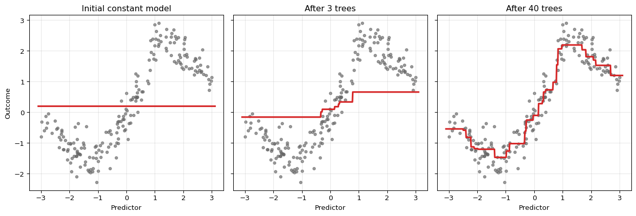
The ensemble starts as a constant. With each iteration, the fit becomes more refined because the next tree is trained on what the current ensemble still gets wrong.
Why Small Trees Are Used
Boosting usually uses shallow trees rather than deep ones. A tree of depth 1 is a stump and captures a single threshold effect. A tree of depth 2 or 3 can capture low-order interactions. This is deliberate regularization:
- shallow trees make each correction simple
- many simple corrections can approximate a complicated function
- restricting tree depth reduces the risk of overfitting each stage
This stagewise logic is one reason boosting performs well on tabular data when the regression function has low- to moderate-order interactions.
12.5 General Gradient Boosting
Gradient boosting extends beyond squared loss by replacing the residual with the negative gradient of a differentiable loss. Suppose the objective is
\[ \sum_{i=1}^n \ell(y_i, F(x_i)), \]
where \(\ell\) is differentiable with respect to the fitted value \(F(x_i)\). Then the pseudo-residual at iteration \(m\) is
\[ r_{im} = - \left. \frac{\partial \ell(y_i, F(x_i))}{\partial F(x_i)} \right|_{F=\hat F_{m-1}}. \]
The next tree is fit to these pseudo-residuals, and the ensemble is updated in the direction of steepest descent in function space. That is why the method is called gradient boosting.
To see the gradient structure precisely, think of \(F\) as a vector \((F(x_1), \ldots, F(x_n))^\top \in \mathbb{R}^n\), where each coordinate is the fitted value at one training observation. The total loss is a function of this vector, \(L(F) = \sum_{i=1}^n \ell(y_i, F(x_i))\) — the same training objective introduced for squared loss in Section 12.4, now written for a general \(\ell\) — and the \(i\)-th coordinate of its negative gradient at \(\hat F_{m-1}\) is exactly \(r_{im}\). Boosting cannot step directly in this direction, because the result would be \(n\) numbers with no way to generalize to new observations. Instead, each tree \(\hat{h}_m\) approximates the negative gradient within a structured, tree-shaped function class. Fitting a tree to the pseudo-residuals is therefore fitting a generalizable approximation to the steepest-descent direction.
Refining the leaf values. Fitting a least-squares tree to the pseudo-residuals serves to determine the split structure — the partition of the predictor space into leaves \(R_{jm}\) (the \(j\)-th leaf of the tree fit at iteration \(m\)) — but the least-squares leaf means need not be the loss-optimal constants on the scale of \(\ell\). The loss-optimal leaf values are obtained by a separate one-dimensional minimization within each leaf,
\[ \gamma_{jm} = \arg\min_{\gamma} \sum_{i:\, x_i \in R_{jm}} \ell\big(y_i,\, \hat F_{m-1}(x_i) + \gamma\big), \]
after which the update becomes \(\hat F_m = \hat F_{m-1} + \nu \sum_j \gamma_{jm} \mathbf{1}\{x \in R_{jm}\}\) rather than \(\hat F_{m-1} + \nu \hat h_m\). For the squared-error case the two coincide — the minimizing \(\gamma_{jm}\) is just the mean pseudo-residual in the leaf — so the distinction only matters for general losses such as the log-odds-scale Bernoulli loss below. This per-leaf line search is Friedman’s (J. H. Friedman 2001) TreeBoost refinement.
Classification with Bernoulli Log-Loss
For binary outcomes, write
\[ p_i = \sigma(F(x_i)) = \frac{1}{1 + e^{-F(x_i)}}, \]
where \(F(x_i)\) is now a log-odds score rather than a probability directly. The Bernoulli log-loss is
\[ \ell(y_i, F(x_i)) = - y_i \log p_i - (1-y_i)\log(1-p_i). \]
Differentiating gives
\[ \frac{\partial \ell}{\partial F(x_i)} = p_i - y_i, \]
so the negative gradient is
\[ r_{im} = y_i - p_i. \]
Classification boosting therefore retains the residual structure, but the residual is on the probability scale (\(y_i \in \{0,1\}\) minus \(p_i \in (0,1)\)) rather than on the outcome scale.
This is exactly a case where the leaf-value refinement above matters: the tree fit to the pseudo-residuals \(r_{im} = y_i - p_i\) fixes only the splits, and because Bernoulli log-loss is not squared error, the leaf constants are then set by the per-leaf line search \(\gamma_{jm}\) rather than by the mean residual in the leaf. That minimization has no closed form here, so implementations take a single Newton step, \(\gamma_{jm} = \big(\sum_{i:\, x_i \in R_{jm}} (y_i - p_i)\big) \big/ \big(\sum_{i:\, x_i \in R_{jm}} p_i(1-p_i)\big)\), using the gradient \(p_i - y_i\) and the curvature \(p_i(1-p_i)\) evaluated at the current probabilities.
Connection to Cross-Entropy
For classification, boosting with Bernoulli log-loss is minimizing cross-entropy, i.e. the negative log-likelihood of a Bernoulli model. This links boosting directly to the MLE-as-KL discussion: fitting the boosted classifier means reducing the discrepancy between observed class outcomes and predicted event probabilities.
AdaBoost as Exponential-Loss Boosting
The general gradient boosting framework unifies algorithms that were developed independently. AdaBoost, introduced by Freund and Schapire (1997) before the gradient boosting connection was made explicit, can be recovered as a special case by choosing exponential loss. The statistical view of AdaBoost as additive logistic regression — and the equivalence between its weighting rule and exponential-loss gradient descent — was made rigorous by J. Friedman, Hastie, and Tibshirani (2000), which remains the canonical reference for the equivalence.
For binary classification with \(y_i \in \{-1, +1\}\), define
\[ \ell(y_i, F(x_i)) = e^{-y_i F(x_i)}. \]
The negative gradient at the current fit is
\[ r_{im} = -\left.\frac{\partial \ell(y_i, F(x_i))}{\partial F(x_i)}\right|_{F=\hat F_{m-1}} = y_i \, e^{-y_i \hat F_{m-1}(x_i)}. \]
Writing \(w_{im} = e^{-y_i \hat F_{m-1}(x_i)}\), the pseudo-residual is \(r_{im} = y_i w_{im}\). Since \(y_i \in \{-1,+1\}\), fitting a tree to these pseudo-residuals is equivalent to fitting a weighted classifier with weight \(w_{im}\) on observation \(i\). Observations that are currently misclassified — those for which \(y_i \hat F_{m-1}(x_i) < 0\) — have \(w_{im} > 1\), so the next tree is directed toward the current mistakes. This is exactly the AdaBoost observation-reweighting step.
The exponential-loss framing also reveals a limitation: \(w_{im}\) grows without bound when an observation is persistently and confidently misclassified. A single outlier can eventually dominate the loss and distort subsequent trees. By contrast, the Bernoulli log-loss gradient \(p_i - y_i\) is bounded in \((-1, 1)\), so the weight placed on any single observation is capped. This robustness is one reason log-loss is generally preferred over exponential loss in econometric applications, where outcomes can have heavy tails or influential observations.
Question for Reflection
AdaBoost and gradient boosting with log-loss both iteratively correct current mistakes. Why might you still prefer log-loss when forecasting binary recession indicators from macroeconomic data, even if both methods reached similar validation accuracy?
Suggested Answer
Macroeconomic time series contain unusual observations — financial crises, pandemic quarters — that are influential precisely because they are rare and extreme. Under exponential loss, a persistently misclassified recession quarter receives an exponentially growing weight, so subsequent trees are pulled toward fitting that single observation rather than improving predictions broadly. Log-loss assigns a bounded gradient to each observation, so no single quarter can disproportionately dominate the boosting path. In a setting where rare events matter but should not dictate the entire model, that boundedness is a meaningful practical advantage.
12.6 Regularization in Boosting
Boosting can keep refining the fit indefinitely. That is why regularization is essential, not optional.
Learning Rate
The learning rate \(\nu\) shrinks each update:
\[ \hat F_m(x) = \hat F_{m-1}(x) + \nu \hat h_m(x). \]
Smaller \(\nu\) means:
- slower learning
- more trees needed
- often better generalization, because the fit evolves more cautiously
This is called shrinkage. The interaction between \(\nu\) and the optimal number of trees \(M\) is roughly reciprocal: a smaller \(\nu\) requires more iterations to reach the same training risk, so halving \(\nu\) approximately doubles the optimal \(M\) chosen by validation (Zhang and Yu 2005). The product \(\nu \cdot M\) behaves like a complexity budget, which is the sense in which shrinkage acts as a regularization device.
Number of Trees
The number of iterations \(M\) controls how long the algorithm keeps refining the fit.
- too few trees can underfit
- too many trees can eventually overfit
- the optimal \(M\) is usually chosen by validation or early stopping — that is, by halting the number of boosting iterations \(M\) at the point where validation error is minimized (see Section 12.7)
Tree Depth
Depth controls interaction order.
- depth 1: additive threshold effects only
- depth 2: two-way interactions can appear
- deeper trees: more complex local interactions, but more risk of overfitting
Subsampling
Some boosting implementations fit each new tree on a random subsample of the data rather than the full sample. This is called stochastic gradient boosting (J. H. Friedman 2002).
Subsampling can:
- reduce variance
- improve robustness
- speed computation
At the cost of introducing additional randomness into the stagewise updates.
Monotonicity Constraints
Sometimes the econometrician has credible prior knowledge about the sign of a predictive relationship even if the rest of the conditional mean is complicated. For example, one might regard it as implausible that a higher debt-service burden should lower predicted default risk, or that a tighter financial-conditions index should lower predicted recession risk, all else equal. A monotonicity constraint imposes exactly such a shape restriction on the fitted function.
In a tree-ensemble model, this means restricting the fitted prediction to move only in one direction as a chosen predictor increases, holding the other predictors fixed. The idea is not unique to boosting, but it is especially prominent in modern boosted-tree implementations because it fits naturally into the broader regularization toolkit. This does not make the model structural or causal. It is better understood as a regularization device that uses economic theory to rule out locally implausible wiggles in the prediction surface.
When the sign restriction is well founded, monotonicity constraints can improve credibility, stabilize partial-effect summaries, and prevent the ensemble from fitting noise in directions that contradict economic reasoning. But they are not free. If the true conditional relationship is non-monotone, changes sign across regimes, or is only monotone after conditioning on variables the model does not include, the constraint can introduce systematic misspecification.
How the constraint is enforced. Inside each tree, a split on a constrained feature is accepted only if the resulting child fitted values respect the sign pattern: for an increasing constraint, the left child’s mean must not exceed the right child’s. To ensure the constraint holds globally and not just locally at each split, modern implementations propagate bounds through the tree: when a node is split on feature \(j\), the fitted values in its children are restricted to an interval computed from the ancestor path, so that even splits on other features cannot eventually produce leaves that violate the monotone ordering across the full predictor space. Splits that would violate the constraint are never taken. This is a hard restriction on the function class, not a penalty added to the loss.
In scikit-learn. The histogram-based gradient-boosting estimator HistGradientBoostingRegressor accepts a monotonic_cst argument with one integer per feature: +1 for increasing, -1 for decreasing, and 0 for no constraint. For three predictors where the first is required to enter monotonically increasing:
from sklearn.ensemble import HistGradientBoostingRegressor

model = HistGradientBoostingRegressor(
    monotonic_cst=[1, 0, 0],
    max_iter=500,
    learning_rate=0.05,
)
See the scikit-learn example Monotonic Constraints for a visual comparison of constrained and unconstrained fits and a full working API example.
Implementation Note: XGBoost
XGBoost (Chen and Guestrin 2016) is an optimized implementation family for gradient-boosted trees. Relative to the basic algorithm in this chapter, it adds engineering and regularization features such as efficient split search, L1/L2-style penalties, sparse or missing-value handling, monotone constraints, and scalable training. The econometric interpretation remains the same: it is still a tuned predictive tree ensemble, so validation design and the information set are central.
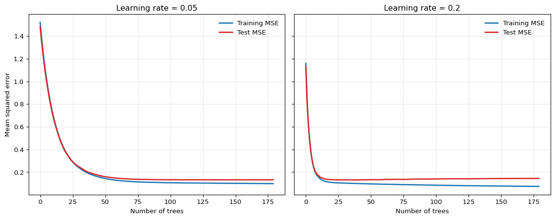
The smaller learning rate often gives a flatter, more forgiving test-error profile, while the larger learning rate improves more quickly but can overfit earlier.
Question for Reflection
If two boosted models have similar validation error, what evidence from the validation curve would justify the small-learning-rate, many-tree model, and what evidence would justify the larger-learning-rate, fewer-tree model?
Suggested Answer
A small learning rate with many trees is better supported when the validation curve is flatter and overfitting appears later along the boosting path. A larger learning rate with fewer trees is better supported when the time-ordered validation curve is genuinely similar but the model reaches that performance with fewer boosting steps and lower computational cost. The comparison should be based on validation over the relevant forecast origins, not on in-sample fit.
The same qualitative pattern appears on actual macroeconomic data. Figure 12.3 shows training and validation MSE curves for annualized GDP growth in quarter \(t+1\) from FRED-QD, using five predictors dated quarter \(t\) — GDP growth, inflation, the term spread, log VIX, and the unemployment rate — and a time-ordered 75/25 split.1 With a small learning rate, the validation curve declines gradually and remains relatively flat; with a large learning rate, validation error reaches its minimum early and then begins to rise — the overfitting signal that early stopping is designed to detect. The absolute MSE values are large relative to the synthetic example because quarterly GDP growth is genuinely difficult to forecast: the 2020 contraction alone generates residuals of tens of annualized percentage points, which dominate the average squared error.
Show the code
import numpy as np
import pandas as pd
import matplotlib.pyplot as plt
from sklearn.ensemble import GradientBoostingRegressor

raw = pd.read_csv("data/fred_qd_current.csv")
fred_qd = raw.iloc[2:].copy()
fred_qd["sasdate"] = pd.to_datetime(fred_qd["sasdate"])
for col in fred_qd.columns:
    if col != "sasdate":
        fred_qd[col] = pd.to_numeric(fred_qd[col], errors="coerce")
fred_qd = fred_qd.sort_values("sasdate").reset_index(drop=True)

gdp_growth  = 400 * np.log(fred_qd["GDPC1"]).diff()
inflation   = 400 * np.log(fred_qd["CPIAUCSL"]).diff()
term_spread = fred_qd["GS10"] - fred_qd["TB3MS"]
log_vix     = np.log(fred_qd["VIXCLSx"])

macro = pd.DataFrame({
    "y":           gdp_growth.shift(-1),
    "gdp_lag1":    gdp_growth,
    "infl_lag1":   inflation,
    "spread_lag1": term_spread,
    "vix_lag1":    log_vix,
    "unrate_lag1": fred_qd["UNRATE"],
}).dropna()

feature_cols = ["gdp_lag1", "infl_lag1", "spread_lag1", "vix_lag1", "unrate_lag1"]
split = int(len(macro) * 0.75)
X_train = macro.iloc[:split][feature_cols].values
y_train = macro.iloc[:split]["y"].values
X_test  = macro.iloc[split:][feature_cols].values
y_test  = macro.iloc[split:]["y"].values

configs = [(0.02, "C0"), (0.2, "C3")]
fig, axes = plt.subplots(1, 2, figsize=(12, 4.5), sharey=True)

for (lr, _), ax in zip(configs, axes):
    model = GradientBoostingRegressor(
        n_estimators=250, learning_rate=lr, max_depth=2,
        min_samples_leaf=6, random_state=42,
    )
    model.fit(X_train, y_train)
    train_mse, val_mse = [], []
    for p_tr, p_te in zip(model.staged_predict(X_train), model.staged_predict(X_test)):
        train_mse.append(np.mean((y_train - p_tr) ** 2))
        val_mse.append(np.mean((y_test  - p_te) ** 2))
    ax.plot(train_mse, color="C0", linewidth=2, label="Training MSE")
    ax.plot(val_mse,   color="C3", linewidth=2, label="Validation MSE")
    ax.set_title(f"Learning rate = {lr}")
    ax.set_xlabel("Number of trees")
    ax.grid(True, alpha=0.3)
    ax.legend(frameon=False)

axes[0].set_ylabel("Mean squared error")
plt.tight_layout()
plt.show()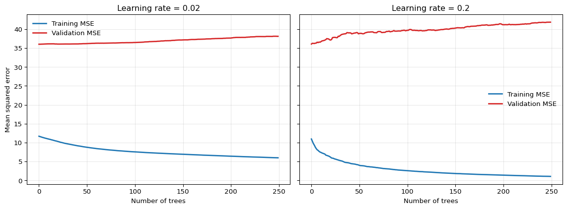
12.7 Early Stopping and Validation
Because boosting can continue to improve the training fit for many iterations, some external criterion is needed to decide when to stop. Early stopping uses a validation set or validation path to choose the number of trees, and it is one of the central regularization devices of boosting — not a minor implementation detail.
Econometric Warning
For forecasting applications, early stopping must be based on time-ordered validation data. Random k-fold validation can leak future information into the tuning process and make boosting appear far stronger than it truly is out of sample.
The validation design should mirror the actual forecast exercise:
- rolling or expanding windows for time series
- group-aware validation for clustered or panel-style dependence
- leakage-safe preprocessing inside each training fold
12.8 Strengths and Limits for Econometric Work
Boosting is among the strongest off-the-shelf methods for tabular prediction. It is effective when:
- nonlinearities are important
- interactions are present but unknown
- there are many candidate predictors
- forecast accuracy matters more than structural interpretability
Strengths
- competitive predictive performance on structured data
- automatic detection of nonlinearities and interactions
- flexible loss functions for means, probabilities, and other targets
- regularization knobs that can be tuned to the signal-to-noise environment
Limitations
- sensitive to hyperparameter tuning and validation design
- no natural extrapolation beyond the support of the training data
- slower and less transparent than a single tree
- variable importance and partial-effect summaries remain predictive, not causal
Like random forests, boosted trees should be understood as flexible predictive approximators, not as identification strategies.
12.9 Summary
Key Takeaways
- Gradient boosting builds an additive tree ensemble sequentially, with each new tree correcting the current ensemble.
- Under squared loss, the pseudo-residuals are ordinary residuals, so boosting repeatedly fits trees to what the current model still misses.
- Under general differentiable losses, boosting follows the negative gradient of the loss in function space; for Bernoulli log-loss, the pseudo-residual is \(y-p\).
- Learning rate, number of trees, tree depth, subsampling, and early stopping are the key regularization devices.
- Boosting is among the most effective methods for econometric prediction on tabular data, but honest validation is essential, especially in time-series applications.
Common Pitfalls
- Using a large learning rate because it improves training loss quickly.
- Choosing the number of trees from a validation scheme that leaks future information.
- Forgetting that tree depth controls interaction complexity.
- Reading boosted-tree importance measures as structural or causal evidence.
- Expecting boosted trees to extrapolate smooth trends outside the training support.
12.10 Exercises
Exercise 12.1: First Step of Gradient Boosting with Shrinkage
Suppose these are four monthly observations from a small forecasting exercise in which \(y_i\) denotes next-month output growth and \(x_i\) is a leading indicator. You observe:
\[ (x_i, y_i) = (1,2), (2,3), (3,2.5), (4,5). \]
Consider squared-error boosting with decision stumps as weak learners. Let the learning rate be \(\nu = 0.4\).
- Briefly explain the idea of gradient boosting under squared loss.
- Compute the initial model \(F_0(x)\) and the residuals \(r_i = y_i - F_0(x_i)\).
- Fit the optimal first stump \(h_1(x)\) by checking the candidate split points \(1.5\), \(2.5\), and \(3.5\).
- Write the updated model \[ F_1(x) = F_0(x) + 0.4\, h_1(x). \] Compute the fitted values at the four training points.
- Compute the training SSE of \(F_1\). Compare it with the training SSE that would result from taking the full step \(\nu=1\). Why can a smaller learning rate still be useful in practice?
Exam level: suitable as-is. The exercise combines boosting mechanics, shrinkage, and the regularization interpretation of the learning rate.
Hint for Part 2
Under squared loss, the best constant predictor is the sample mean.
Hint for Part 3
For each candidate split, compute the mean residual in the left and right leaf and then the residual SSE.
Hint for Part 5
A smaller learning rate usually gives a worse fit after one step, but that is not the right comparison. Boosting is a multi-step procedure.
Solution
Part 1: Core idea
Under squared loss, boosting starts from a simple predictor and then repeatedly fits a weak learner to the current residuals. Each new tree corrects part of the remaining error.
Part 2: Initial model and residuals
The initial model is the sample mean:
\[ F_0(x)=\bar y=\frac{2+3+2.5+5}{4}=3.125. \]
Therefore the residuals are
\[ r = (-1.125,\,-0.125,\,-0.625,\,1.875). \]
Part 3: Best first stump
Check the three candidate cutoffs.
For split \(1.5\):
- left mean residual: \(-1.125\)
- right mean residual: \(\frac{-0.125-0.625+1.875}{3}=0.375\)
Residual SSE:
\[ 0 + (-0.125-0.375)^2 + (-0.625-0.375)^2 + (1.875-0.375)^2 = 3.5. \]
For split \(2.5\):
- left mean residual: \(\frac{-1.125-0.125}{2}=-0.625\)
- right mean residual: \(\frac{-0.625+1.875}{2}=0.625\)
Residual SSE:
\[ (-1.125+0.625)^2 + (-0.125+0.625)^2 + (-0.625-0.625)^2 + (1.875-0.625)^2 = 3.625. \]
For split \(3.5\):
- left mean residual: \(\frac{-1.125-0.125-0.625}{3}=-0.625\)
- right mean residual: \(1.875\)
Residual SSE:
\[ (-1.125+0.625)^2 + (-0.125+0.625)^2 + (-0.625+0.625)^2 + (1.875-1.875)^2 = 0.5. \]
So the best first stump is
\[ h_1(x)= \begin{cases} -0.625, & x \leq 3.5, \\ 1.875, & x > 3.5. \end{cases} \]
Part 4: Shrinkage update
With \(\nu=0.4\),
\[ F_1(x)=F_0(x)+0.4\,h_1(x). \]
Therefore
\[ F_1(x)= \begin{cases} 3.125 + 0.4(-0.625)=2.875, & x \leq 3.5, \\ 3.125 + 0.4(1.875)=3.875, & x > 3.5. \end{cases} \]
So the fitted values at the four training points are
\[ (2.875,\ 2.875,\ 2.875,\ 3.875). \]
Part 5: Training SSE and interpretation
The training SSE is
\[ (2-2.875)^2 + (3-2.875)^2 + (2.5-2.875)^2 + (5-3.875)^2 = 2.1875. \]
If instead \(\nu=1\), then
\[ F_1(x)= \begin{cases} 2.5, & x \leq 3.5, \\ 5, & x > 3.5, \end{cases} \]
and the resulting SSE is
\[ (2-2.5)^2 + (3-2.5)^2 + (2.5-2.5)^2 + (5-5)^2 = 0.5. \]
So after one step, the full update fits the training sample better. But a smaller learning rate can still be useful because it regularizes the path of the algorithm. With many steps, cautious updates often generalize better out of sample than aggressive early corrections.
Exercise 12.2: Bernoulli Log-Loss and Early Stopping
Consider binary outcomes \(y_i \in \{0,1\}\) and a boosting model with score \(F(x_i)\) and probability
\[ p_i = \sigma(F(x_i)) = \frac{1}{1+e^{-F(x_i)}}. \]
The Bernoulli log-loss for observation \(i\) is
\[ \ell(y_i,F(x_i)) = - y_i \log p_i - (1-y_i)\log(1-p_i). \]
- Show that \[ \frac{\partial \ell(y_i,F(x_i))}{\partial F(x_i)} = p_i - y_i. \] Conclude that the pseudo-residual is \(r_i = y_i - p_i\).
- Suppose the initial model is a constant, \(F_0(x)\equiv c\). Show that the value minimizing the total log-loss satisfies \[ \sigma(c)=\bar y, \] and hence \[ c = \log\left(\frac{\bar y}{1-\bar y}\right). \]
- For the sample \(y=(1,1,0,1)\), compute \(\bar y\), the optimal initial constant \(F_0\), the implied initial probability \(p_i\), and the pseudo-residuals.
Exam level: suitable as-is. Parts 1-3 derive the classification gradients formally.
Hint for Part 1
Differentiate through the logistic link: \(\sigma'(z)=\sigma(z)(1-\sigma(z))\).
Hint for Part 2
Differentiate the total loss with respect to the constant \(c\) and set the derivative equal to zero.
Solution
Part 1: Derivative of log-loss
Write \(p_i=\sigma(F_i)\) with \(F_i=F(x_i)\). Then
\[ \ell_i = -y_i \log p_i - (1-y_i)\log(1-p_i). \]
Differentiate with respect to \(F_i\):
\[ \frac{\partial \ell_i}{\partial F_i} = -y_i \frac{1}{p_i}\frac{\partial p_i}{\partial F_i} - (1-y_i)\frac{1}{1-p_i}\left(-\frac{\partial p_i}{\partial F_i}\right). \]
Since \(\frac{\partial p_i}{\partial F_i}=p_i(1-p_i)\), this becomes
\[ \frac{\partial \ell_i}{\partial F_i} = -y_i(1-p_i) + (1-y_i)p_i = p_i - y_i. \]
Therefore the negative gradient is
\[ r_i = -\frac{\partial \ell_i}{\partial F_i} = y_i - p_i. \]
Part 2: Optimal constant initial model
If \(F_0(x)\equiv c\), then every observation has the same probability \(p=\sigma(c)\). The total loss is
\[ L(c)= -\sum_{i=1}^n \left[y_i \log p + (1-y_i)\log(1-p)\right]. \]
From Part 1, the derivative with respect to \(c\) is
\[ \frac{dL}{dc} = \sum_{i=1}^n (p - y_i) = np - \sum_{i=1}^n y_i. \]
Setting this equal to zero gives
\[ p = \frac{1}{n}\sum_{i=1}^n y_i = \bar y. \]
Since \(p=\sigma(c)\),
\[ \sigma(c)=\bar y. \]
Applying the logit transformation,
\[ c = \log\left(\frac{\bar y}{1-\bar y}\right). \]
Part 3: Numerical example
For \(y=(1,1,0,1)\),
\[ \bar y = \frac{3}{4} = 0.75. \]
Hence
\[ F_0 = \log\left(\frac{0.75}{0.25}\right)=\log 3 \approx 1.099. \]
The implied initial probability is
\[ p_i = \sigma(F_0)=0.75 \qquad \text{for all } i. \]
So the pseudo-residuals are
\[ r = (1-0.75,\ 1-0.75,\ 0-0.75,\ 1-0.75) = (0.25,\ 0.25,\ -0.75,\ 0.25). \]
12.11 References
Chen, Tianqi, and Carlos Guestrin. 2016. “XGBoost: A Scalable Tree Boosting System.” In Proceedings of the 22nd ACM SIGKDD International Conference on Knowledge Discovery and Data Mining, 785–94. https://doi.org/10.1145/2939672.2939785.
Freund, Yoav, and Robert E. Schapire. 1997. “A Decision-Theoretic Generalization of On-Line Learning and an Application to Boosting.” Journal of Computer and System Sciences 55 (1): 119–39. https://doi.org/10.1006/jcss.1997.1504.
Friedman, Jerome H. 2001. “Greedy Function Approximation: A Gradient Boosting Machine.” Annals of Statistics 29 (5): 1189–1232.
———. 2002. “Stochastic Gradient Boosting.” Computational Statistics & Data Analysis 38 (4): 367–78. https://doi.org/10.1016/S0167-9473(01)00065-2.
Friedman, Jerome, Trevor Hastie, and Robert Tibshirani. 2000. “Additive Logistic Regression: A Statistical View of Boosting.” Annals of Statistics 28 (2): 337–407. https://doi.org/10.1214/aos/1016218223.
Zhang, Tong, and Bin Yu. 2005. “Boosting with Early Stopping: Convergence and Consistency.” Annals of Statistics 33 (4): 1538–79. https://doi.org/10.1214/009053605000000255.
Footnotes
This is a pedagogical final-vintage FRED-QD example. A full real-time GDP forecasting evaluation would also need to account for release calendars and data revisions.↩︎