Under active development. A stable version is expected in November 2026. Feedback is very welcome.

7 LSTM Networks

7.1 Overview

The previous chapter showed the central weakness of a plain RNN: the hidden state is recursively updated, but the gradients used for learning can vanish as they are propagated backward through many time steps. Long Short-Term Memory (LSTM) networks were designed to address precisely this problem.

The key innovation is the introduction of a dedicated cell state \(C_t\), which acts as a more stable memory path through time. This memory path is controlled by gates: small neural-network components that decide what information to retain, what new information to add, and what part of the internal memory to expose as the hidden state.

For econometricians, LSTMs are useful when the relevant predictive state may evolve over time and depend on information from more than only the most recent observations. Examples include asset pricing with time-varying macroeconomic states, macroeconomic forecasting with long predictor histories, and volatility or risk forecasting with persistent regimes.

For optional visual intuition, this blog post gives a detailed informal discussion of LSTMs.

7.2 Roadmap

We first introduce the LSTM cell state, hidden state, and gates.
We then work through the LSTM update equations and notation.
Next, we explain why the cell state improves gradient flow relative to a plain RNN.
We discuss when the additional complexity of an LSTM is useful in econometric forecasting.
We close with a research application in asset pricing, key takeaways, common pitfalls, and a manual forward-pass exercise.

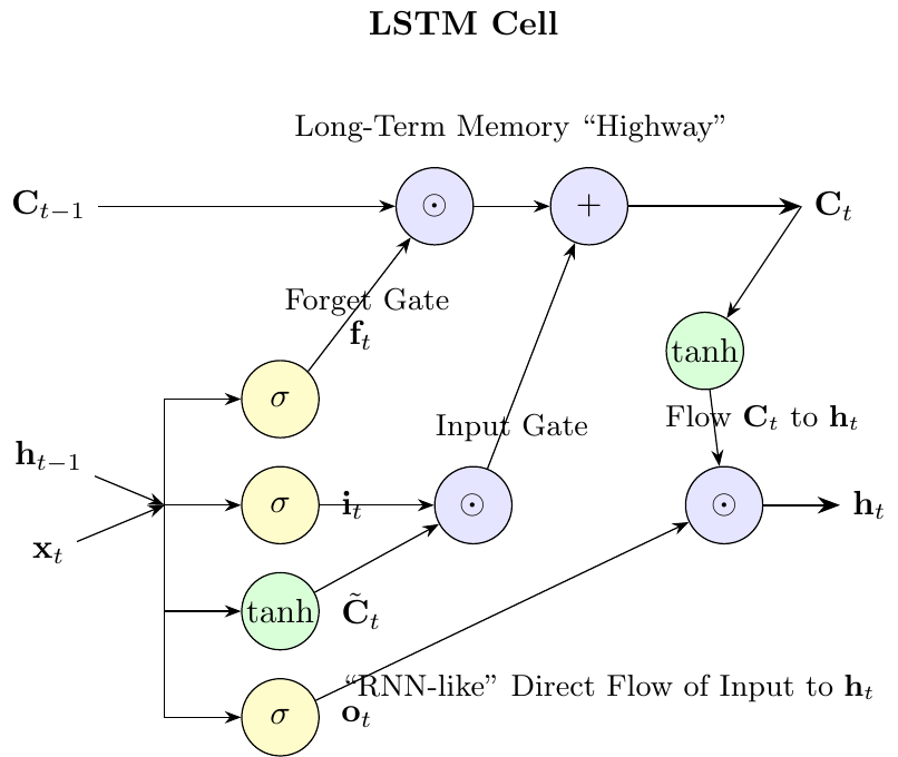
7.3 LSTM Architecture and Notation

Long Short-Term Memory (LSTM) networks introduced by Hochreiter and Schmidhuber (1997) extend vanilla RNNs by introducing a gating mechanism that controls long-term information flow. Before diving into the mathematical details, we need to establish the notation because LSTMs update several quantities at each time step.

At each time step \(t\), an LSTM cell maintains:

Input: \(x_t \in \mathbb{R}^D\), the current input vector
Hidden state: \(h_t \in \mathbb{R}^H\), the output of the LSTM cell, similar to RNN hidden states
Cell state: \(C_t \in \mathbb{R}^H\), the internal memory of the LSTM cell

The LSTM uses four different gates and candidate values (all in \(\mathbb{R}^H\)):

Forget gate: \(f_t\), controls what information to retain from or discard from the previous cell state
Input gate: \(i_t\), controls what new information to store in the cell state
Candidate values: \(\tilde{C}_t\), new candidate information that could be added to the cell state
Output gate: \(o_t\), controls what parts of the cell state to output as the hidden state

Update Equations and Weight Matrices

Let \(\sigma\) denote the sigmoid function. The LSTM cell state and hidden state are updated according to:

\begin{aligned} f_t &= \sigma(W_f \cdot [h_{t-1}, x_t] + b_f) \quad \text{(forget gate)} \\ i_t &= \sigma(W_i \cdot [h_{t-1}, x_t] + b_i) \quad \text{(input gate)} \\ \tilde{C}_t &= \tanh(W_c \cdot [h_{t-1}, x_t] + b_c) \quad \text{(candidate values)} \\ C_t &= f_t \odot C_{t-1} + i_t \odot \tilde{C}_t \quad \text{(cell state update)} \\ o_t &= \sigma(W_o \cdot [h_{t-1}, x_t] + b_o) \quad \text{(output gate)} \\ h_t &= o_t \odot \tanh(C_t) \quad \text{(hidden state)} \end{aligned}

Each gate and the candidate values are computed using their own weight matrices and bias vectors. Since the input to each is the concatenation \([h_{t-1}, x_t] \in \mathbb{R}^{H+D}\), the dimensions are:

\(W_f, W_i, W_c, W_o \in \mathbb{R}^{H \times (H+D)}\): weight matrices
\(b_f, b_i, b_c, b_o \in \mathbb{R}^H\): bias vectors

Key symbols:

\(\odot\): element-wise multiplication (Hadamard product)
\(\cdot\): dot product (matrix-vector multiplication)
\([h_{t-1}, x_t]\): concatenation of the previous hidden state and current input

The Gating Mechanism

A “gate” is a mechanism to selectively let information pass. In LSTMs, this is achieved by combining a sigmoid activation function with element-wise multiplication. The sigmoid function squashes any input to a value between 0 and 1. This output vector then acts as a gate keeper:

A gate value of 0 means “let nothing through” (closed gate).
A gate value of 1 means “let everything through” (open gate).
A value between 0 and 1 means “let something through (partially open/closed).”

The detailed flow diagram can be found below in Figure 7.1.

7.4 Gradient Flow in LSTMs

One of the key innovations of LSTMs is how they address the vanishing gradient problem in vanilla RNNs. The solution lies in the design of the cell state and its update mechanism.

The Cell State as a Gradient Highway

The LSTM introduces a separate cell state \(C_t\) that follows the update rule:

C_t = f_t \odot C_{t-1} + i_t \odot \tilde{C}_t

This creates an additive path for information to move forward and for gradients to flow backward, unlike the purely multiplicative path in vanilla RNNs. The cell state acts as a “highway” that can carry gradient information across many time steps.

Mathematical Analysis of Gradient Flow

To understand how gradients flow through the cell state, let’s compute the partial derivative:

\frac{\partial C_t}{\partial C_{t-1}} = f_t

For gradient flow over multiple time steps from time \(T\) back to time \(t\):

\frac{\partial C_T}{\partial C_t} = \frac{\partial C_T}{\partial C_{T-1}} \frac{\partial C_{T-1}}{\partial C_{T-2}} \cdots \frac{\partial C_{t+1}}{\partial C_t} = \prod_{k=t+1}^T f_k

Key Differences from Vanilla RNNs

The gradient flow in LSTMs differs fundamentally from vanilla RNNs in three crucial ways:

Additive Structure: The cell state update is additive (\(C_t = f_t \odot C_{t-1} + \text{new information}\)) rather than the multiplicative structure in RNNs (\(h_t = \tanh(W_h h_{t-1} + \ldots)\)).
Controlled Forgetting: The forget gate \(f_t \in [0,1]\) (due to sigmoid activation) controls how much of the previous cell state to retain. When \(f_t \approx 1\), gradients flow almost unimpeded.
Weight-Independent Gradients: The gradient magnitude depends only on forget gate values, not on weight matrices and their norms.

Comparison of Gradient Expressions

\begin{aligned} \text{Vanilla RNN:} \quad &\frac{\partial h_T}{\partial h_t} = \prod_{k=t+1}^T \frac{\partial h_k}{\partial h_{k-1}} = \prod_{k=t+1}^T W_h \cdot \text{diag}(\tanh'(\cdot)) \\ \text{LSTM:} \quad &\frac{\partial C_T}{\partial C_t} = \prod_{k=t+1}^T f_k \end{aligned}

In RNNs, each factor involves the weight matrix \(W_h\) and the derivative of the activation function, leading to exponential decay or explosion. In LSTMs, the factors are simply the forget gate values, which the network can learn to control.

Selective Memory Through Adaptive Gating

The forget gate \(f_t = \sigma(W_f \cdot [h_{t-1}, x_t] + b_f)\) provides adaptive memory control:

Selective Forgetting: When the network determines that previous information is no longer relevant, it can set \(f_t \approx 0\) to “forget” the cell state.
Long-term Retention: When information should be preserved, the network can set \(f_t \approx 1\), allowing gradients to flow backward with minimal attenuation.
Context-Dependent Decisions: The forget gate’s dependence on both \(h_{t-1}\) and \(x_t\) allows the network to make context-aware decisions about what to remember or forget.

The Gradient Highway Effect

When the forget gate learns to be close to 1 for important long-term dependencies:

\frac{\partial C_T}{\partial C_t} = \prod_{k=t+1}^T f_k \approx 1^{T-t} = 1

This means gradients can flow backward through many time steps without significant attenuation, enabling the learning of long-term dependencies.

Key Insight: Unlike vanilla RNNs where gradient flow is strongly shaped by repeated multiplication with recurrent weight matrices, LSTMs learn when to allow gradients to flow through the forget gates. This learned control mechanism is what makes LSTMs useful for sequences with complex temporal dependence.

7.5 LSTM vs. Standard RNN

Aspect	Standard RNN	LSTM
Memory Capability	Short-term only	Capable of learning long-term dependencies
Gradient Flow	Multiplicative (via weight matrices)	Additive (via cell state)
Vanishing Gradients	Highly susceptible	Largely mitigated by the “gradient highway”
Parameters	\(O(H^2)\)	\(O(4H^2)\) (four sets of weights)
Computational Cost	Low	~4x higher per cell

When to use LSTM:

Forecasting tasks where information from distant observations plausibly matters, such as macroeconomic state dynamics or asset-pricing applications with persistent risk states.
Settings where validation performance justifies the extra parameters and computational cost.

When a standard RNN might suffice:

Problems with very short sequences where long-term memory is not needed.
When computational resources are extremely limited.

Question for Reflection

Suppose an LSTM is trained on monthly data and the forget gate learns values close to 1 for one hidden dimension and close to 0 for another. Using the gradient expression \(\partial C_T / \partial C_t = \prod_{k=t+1}^{T} f_k\), which dimension can transmit information across many time steps, and what happens to the gradient signal in the other dimension?

7.6 Research Application: Deep Learning in Asset Pricing

To see how LSTMs are used in state-of-the-art econometric research, consider the asset-pricing framework of Chen, Pelger, and Zhu (2024).

The Core Research Question

The paper asks a fundamental question in finance: Can neural networks better model the relationship between firm characteristics and future stock returns?

The Traditional Approach (Linear Factor Models): Assumes a simple linear relationship, \(\mathbb{E}[r_{i,t+1}] = \beta_0 + \sum_k \beta_k \cdot \text{characteristic}_{i,t,k}\). This is restrictive, as it ignores non-linearities (e.g., threshold effects) and complex interactions between characteristics (e.g., value investing working best when momentum is low).
The Deep Learning Approach: Lets a neural network learn the functional form directly from the data: \(\mathbb{E}[r_{i,t+1}] = f(\text{characteristics}_{i,t})\). The network can approximate nonlinear functions and interactions that are difficult to specify manually.

Framing the Problem for a Neural Network

The task is a large-scale panel data regression, framed as a standard supervised learning problem.

Inputs (\(\mathbf{x}_{i,t}\)): A vector of 94 firm-specific characteristics for stock \(i\) at time \(t\) (e.g., size, value, momentum, profitability).
Target (\(y_{i,t+1}\)): The realized excess return of stock \(i\) in the next month.
Objective: Train a neural network \(f_\theta\) to minimize the Mean Squared Error (MSE) between predicted and realized returns over a large dataset of all US stocks from 1957 to 2016. \[ \min_\theta \frac{1}{N \cdot T} \sum_{i,t} (r_{i,t+1} - f_\theta(\mathbf{x}_{i,t}))^2 \]

The trained network \(f_\theta(\cdot)\) is part of the estimated Stochastic Discount Factor (SDF). The important point for this chapter is how the authors use an LSTM to represent time variation in the economic state.

Step 1: A Simple Feed-Forward Network (NN1)

A natural starting point is a standard feedforward neural network to model the cross-sectional relationship.

graph LR
    A["Input Layer<br/>(94 Characteristics)"] --> B["Hidden Layer 1<br/>(32 neurons, ReLU)"]
    B --> C["Hidden Layer 2<br/>(16 neurons, ReLU)"]
    C --> D["Hidden Layer 3<br/>(8 neurons, ReLU)"]
    D --> E["Output Layer<br/>(1 neuron, linear)"]

    style A fill:#e6f2ff,stroke:#333
    style B fill:#fff2e6,stroke:#333
    style C fill:#fff2e6,stroke:#333
    style D fill:#fff2e6,stroke:#333
    style E fill:#ffe6e6,stroke:#333

The depth of the network allows it to learn a hierarchy of features. For example, the first layer might learn to combine basic accounting ratios into a value signal, and a deeper layer could then learn to model the interaction between this value signal and momentum signals.

Step 2: Adding Economic Structure with an LSTM (NN2)

Economic Argument: Asset pricing theory (e.g., ICAPM) suggests that risk premia are not constant; they vary over time with the macroeconomic state.
Problem with NN1: It assumes the pricing function \(f(\cdot)\) is the same every month, ignoring time-series dynamics.
Solution (NN2): Use an LSTM to explicitly model the time-varying economic state. The LSTM processes a sequence of macroeconomic variables (e.g., VIX, T-bill rates), and its hidden state \(\mathbf{h}_t\) becomes a learned representation of the current “macro state.” This state vector is then fed as an additional input to the main feed-forward network.

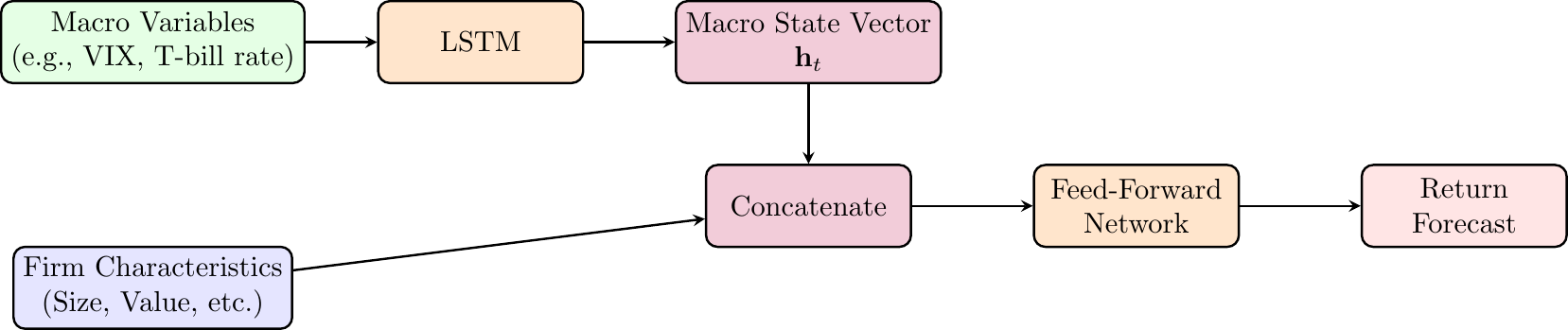
Figure 7.2: LSTM-Based Asset Pricing NN Architecture

This architecture allows the model to learn a state-dependent pricing function:

\mathbb{E}[r_{i,t+1}] = f(\text{characteristics}_{i,t}, \textbf{macro\_state}_t).

Step 3: Enforcing No-Arbitrage

The authors take a final step to enforce the economic constraint of no-arbitrage by using a Generative Adversarial Network (GAN) framework. This advanced technique adjusts the training objective beyond simple MSE to ensure the resulting model is economically consistent. We do not cover GANs in class.

Empirical Results and Conclusions

Performance: The full model (GAN-SDF) achieves an annual out-of-sample Sharpe ratio of approximately 2.6, significantly outperforming linear models (~1.7) and the Fama-French 5-factor model (~0.8).
Explanatory Power: The model explains over 90% of the cross-sectional variation in returns on 46 well-known anomaly portfolios.
Main lesson: The paper demonstrates that combining economic domain knowledge (no-arbitrage constraints, time-varying macro states) with modern machine learning techniques (LSTMs, GANs) yields superior results compared to using either approach in isolation.

7.7 From Recurrent States to Attention

The LSTM cell state \(C_t\) is a fixed-dimensional vector that summarizes the relevant past at each step. Its width \(H\) is chosen once, before training, and does not change with the length of the input sequence. Everything a plain LSTM uses at step \(t\) to forecast must pass through this bottleneck.

This design is efficient, but it has a structural cost. If the predictively relevant past at step \(t\) requires distinguishing fine information from many earlier positions, an \(H\)-dimensional vector has to compress all of it into the same width. For moderately long sequences or for tasks where position-specific information matters — a monetary-policy statement whose meaning depends on whether a given clause appears in paragraph two or paragraph eight, for instance — the bottleneck becomes binding.

The next chapter, Foundation Models for Economic Text and Expectations, introduces a different construction. At each step, instead of pushing the past through a recurrent state, the model explicitly forms a weighted average of representations of all earlier positions, with weights computed from learned similarities. This is the mechanism called self-attention. The advantage over a recurrent state is that nothing is pre-compressed: the set of available inputs at step \(t\) is the entire history, and the model chooses at each step which earlier positions matter. The disadvantage is computational — the number of similarity scores grows quadratically in the sequence length — and for short sequences with strong local dependence an LSTM can still be competitive.

The transition from recurrent states to attention is the single structural change that distinguishes the RNN/LSTM chapters from the foundation-model chapter. We return to it formally in From Words to Representations.

7.8 Summary

Key Takeaways

LSTMs modify the plain RNN state update to reduce the vanishing-gradient problem.
The cell state \(C_t\) provides a more stable path for information and gradients to move through time.
Forget, input, and output gates learn what to retain, what to add, and what to reveal at each time step.
The improvement comes at a cost: an LSTM has several sets of weights and is more computationally expensive than a standard RNN.
In econometric forecasting, LSTMs are most useful when the predictive state is likely persistent and validation performance supports the added complexity.
In asset-pricing applications, an LSTM can be used to represent a time-varying macroeconomic state that conditions the cross-sectional pricing function.

Common Pitfalls

Thinking that LSTMs eliminate all long-run dependence problems; they mitigate vanishing gradients, but still require enough data and careful validation.
Interpreting the LSTM cell state as a directly observed economic state rather than a learned predictive representation.
Using an LSTM when a lagged feed-forward network or simpler time-series model already performs well out of sample.
Forgetting that the gates add parameters, making overfitting a serious concern in small macroeconomic samples.
Evaluating LSTM forecasts with random splits that violate the forecast-origin information set.

7.9 Exercises

Exercise 7.1: Manual LSTM Forward Pass

Consider an LSTM cell with a single unit (no peephole connections) processing one time step. You will compute all gate values, cell state, and hidden state step by step.

Given Parameters:

Forget gate: \(W_f = [0.3, 0.2]\), \(b_f = 0.1\)
Input gate: \(W_i = [0.4, 0.1]\), \(b_i = 0.0\)
Output gate: \(W_o = [0.2, 0.5]\), \(b_o = 0.2\)
Candidate values: \(W_c = [0.6, -0.3]\), \(b_c = 0.0\)

Initial Conditions: - Current input: \(x_1 = 0.5\) - Previous hidden state: \(h_0 = 0.3\) - Previous cell state: \(C_0 = 0.4\)

Tasks:

Compute the forget gate value \(f_1\) using the sigmoid activation function.
Compute the input gate value \(i_1\) using the sigmoid activation function.
Compute the candidate values \(\tilde{C}_1\) using the tanh activation function.
Update the cell state \(C_1\) by combining information from the forget gate, input gate, and candidate values.
Compute the output gate value \(o_1\) using the sigmoid activation function.
Compute the final hidden state \(h_1\) by applying the output gate to the transformed cell state.

Note: Use sigmoid \(\sigma(z) = \frac{1}{1+e^{-z}}\) for gates and \(\tanh\) for candidate values and final hidden state computation.

Exam level. However, the exercise would not be in an exam as it is written here one to one. The skills necessary to solve this exercise can also be tested based on a much simpler network architecture.

Hint 1: Input Vector Construction

For LSTM computations, you need to concatenate the previous hidden state and current input: \([h_{t-1}, x_t] = [h_0, x_1] = [0.3, 0.5]\).

All weight matrices operate on this concatenated vector using dot product: \(W \cdot [h_{t-1}, x_t] + b\).

Hint 2: Gate Computation Order

Compute gates in this order for clarity:

Forget gate (determines what to forget from previous cell state)
Input gate (determines what new information to store)
Candidate values (new information to potentially add)
Cell state update (combine old and new information)
Output gate (determines what to output)
Hidden state (filtered version of cell state)

Hint 3: Key Approximations

Use these approximations to check your work:

\(\sigma(0.29) \approx 0.572\)
\(\sigma(0.17) \approx 0.542\)
\(\sigma(0.51) \approx 0.625\)
\(\tanh(0.03) \approx 0.030\)
\(\tanh(0.245) \approx 0.240\)

Solution

The LSTM equations are:

\begin{aligned} f_t &= \sigma(W_f \cdot [h_{t-1}, x_t] + b_f) \quad \text{(forget gate)} \\ i_t &= \sigma(W_i \cdot [h_{t-1}, x_t] + b_i) \quad \text{(input gate)} \\ \tilde{C}_t &= \tanh(W_c \cdot [h_{t-1}, x_t] + b_c) \quad \text{(candidate values)} \\ C_t &= f_t \odot C_{t-1} + i_t \odot \tilde{C}_t \quad \text{(cell state)} \\ o_t &= \sigma(W_o \cdot [h_{t-1}, x_t] + b_o) \quad \text{(output gate)} \\ h_t &= o_t \odot \tanh(C_t) \quad \text{(hidden state)} \end{aligned}

where \(\sigma(z) = \frac{1}{1+e^{-z}}\) is the sigmoid function.

Given: \(x_1 = 0.5\), \(h_0 = 0.3\), \(C_0 = 0.4\)

The concatenated input vector is \([h_0, x_1] = [0.3, 0.5]\).

Task 1: Forget Gate

\begin{aligned} f_1 &= \sigma(W_f \cdot [0.3, 0.5] + b_f) \\ &= \sigma(0.3 \cdot 0.3 + 0.2 \cdot 0.5 + 0.1) \\ &= \sigma(0.09 + 0.1 + 0.1) \\ &= \sigma(0.29) \approx 0.572 \end{aligned}

Task 2: Input Gate

\begin{aligned} i_1 &= \sigma(W_i \cdot [0.3, 0.5] + b_i) \\ &= \sigma(0.4 \cdot 0.3 + 0.1 \cdot 0.5 + 0.0) \\ &= \sigma(0.12 + 0.05) \\ &= \sigma(0.17) \approx 0.542 \end{aligned}

Task 3: Candidate Values

\begin{aligned} \tilde{C}_1 &= \tanh(W_c \cdot [0.3, 0.5] + b_c) \\ &= \tanh(0.6 \cdot 0.3 + (-0.3) \cdot 0.5 + 0.0) \\ &= \tanh(0.18 - 0.15) \\ &= \tanh(0.03) \approx 0.030 \end{aligned}

Task 4: Cell State Update

\begin{aligned} C_1 &= f_1 \odot C_0 + i_1 \odot \tilde{C}_1 \\ &= 0.572 \cdot 0.4 + 0.542 \cdot 0.030 \\ &= 0.229 + 0.016 \\ &= 0.245 \end{aligned}

Task 5: Output Gate

\begin{aligned} o_1 &= \sigma(W_o \cdot [0.3, 0.5] + b_o) \\ &= \sigma(0.2 \cdot 0.3 + 0.5 \cdot 0.5 + 0.2) \\ &= \sigma(0.06 + 0.25 + 0.2) \\ &= \sigma(0.51) \approx 0.625 \end{aligned}

Task 6: Hidden State

\begin{aligned} h_1 &= o_1 \odot \tanh(C_1) \\ &= 0.625 \cdot \tanh(0.245) \\ &= 0.625 \cdot 0.240 \\ &\approx 0.150 \end{aligned}

Final Results for time step 1:

Forget gate: \(f_1 \approx 0.572\)
Input gate: \(i_1 \approx 0.542\)
Candidate values: \(\tilde{C}_1 \approx 0.030\)
Cell state: \(C_1 \approx 0.245\)
Output gate: \(o_1 \approx 0.625\)
Hidden state: \(h_1 \approx 0.150\)

Key Learning Points:

This exercise demonstrates several important aspects of LSTM computation:

Information Flow Control: Notice how the forget gate (\(f_1 = 0.572\)) moderately retains previous cell state information, while the input gate (\(i_1 = 0.542\)) allows roughly half of the new candidate information to be incorporated.
Cell State as Memory: The cell state update \(C_1 = f_1 \odot C_0 + i_1 \odot \tilde{C}_1\) shows how LSTMs blend old memory (0.229 from previous state) with new information (0.016 from candidates) to maintain long-term dependencies.
Selective Output: The output gate (\(o_1 = 0.625\)) filters what portion of the cell state becomes the hidden state, demonstrating how LSTMs can store information internally without immediately exposing it.
Computational Complexity: Even for a single time step with one unit, LSTMs require computing four different weight-input combinations, highlighting why they are computationally more expensive than simple RNNs.

References

Chen, Luyang, Markus Pelger, and Jason Zhu. 2024. “Deep Learning in Asset Pricing.” Management Science 70 (2): 714–50. https://doi.org/10.1287/mnsc.2023.4695.

Hochreiter, Sepp, and Jürgen Schmidhuber. 1997. “Long Short-Term Memory.” Neural Computation 9 (8): 1735–80. https://doi.org/10.1162/neco.1997.9.8.1735.