Under active development. A stable version is expected in November 2026. Feedback is welcome by email or via GitHub issues.
3 Evaluating Predictive Distributions
3.1 Overview
In many economic and financial applications, predicting a single value (a “point forecast”) is not enough. We often need to understand the full range of possible outcomes and their likelihoods. This requires us to move from point forecasts to distribution forecasts.
For econometricians, this matters whenever decisions depend on tail risk, uncertainty, or the full conditional distribution rather than only the conditional mean. Examples include inflation fan charts, recession-risk assessment, and risk-management quantities such as Value-at-Risk (the loss threshold exceeded only with a given small probability).
This chapter explains how to evaluate such forecasts in a way that rewards honest uncertainty quantification rather than only accurate point predictions.
3.2 Roadmap
- We begin by clarifying the difference between point forecasts and distribution forecasts.
- We then introduce proper scoring rules, the basic tools for evaluating predictive distributions.
- We study the two most important univariate scoring rules in practice: LogS and CRPS.
- We then turn to calibration diagnostics using the Probability Integral Transform (PIT).
- Finally, we connect these ideas back to information theory, especially cross-entropy and KL divergence.
3.3 Distribution Forecasts vs. Point Forecasts
Let’s compare the two approaches:
Point Forecasts:
- Predict a single value, e.g., “tomorrow’s inflation will be 2.5%”.
- This is often the conditional mean or median of the distribution.
- Evaluated using metrics like Mean Squared Error (MSE) or Mean Absolute Error (MAE).
Distribution Forecasts:
- Predict an entire probability distribution for the future outcome, e.g., \(P(Y_{t+1} | \mathcal{F}_t)\), where \(\mathcal{F}_t\) is the information set available at time \(t\) (the forecast origin).
- Provides a complete picture of uncertainty, including variance, skewness, and tail risks.
- More informative for decision-making, such as risk management or policy analysis.
Applications in Economics:
- Inflation Forecasting: Central banks are interested in the probability of inflation exceeding a certain target, not just the single most likely value.
- Risk Management: Financial institutions need to estimate the distribution of potential losses (e.g., Value-at-Risk at multiple risk levels).
- Policy Analysis: Governments need to understand the range of potential impacts of a new policy under uncertainty.
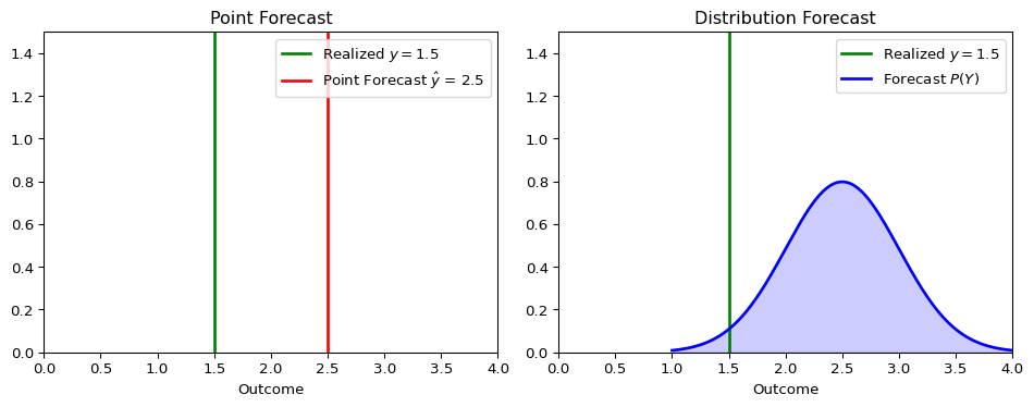
The figure below illustrates the conceptual difference.
A point forecast provides a single best guess, while a distribution forecast provides a richer view of what might happen.
Evaluation Workflow
In practice, evaluating distribution forecasts usually has two components:
- Scoring rules to rank competing forecast models with a single numerical criterion.
- Calibration diagnostics to understand why a forecast distribution is failing.
LogS and CRPS address the first task. PIT histograms address the second.
3.4 Proper Scoring Rules
To evaluate a distribution forecast, we need a metric that assesses the quality of the entire predicted distribution, given the one outcome that actually occurred. This is the role of scoring rules.
A scoring rule \(S(P, y)\) assigns a numerical score to a forecast distribution \(P\) when the outcome \(y\) is realized, just like MSE assigns an error to a point forecast \(\hat y\) and \(y\).
Definition of Proper Scoring Rules
Let \(\mathcal{P}\) be a class of predictive distributions on the outcome space. A scoring rule \(S(P,y)\) assigns a real-valued score to each combination of distribution \(P \in \mathcal{P}\) and outcome \(y\), and we assume throughout that \(\mathbb{E}_{Y \sim F}[S(G,Y)]\) is finite for every \(F, G \in \mathcal{P}\). Under our loss convention (lower is better), \(S\) is proper on \(\mathcal{P}\) if reporting the truth is optimal in expectation:
\[ \mathbb{E}_{Y \sim F}[S(F,Y)] \leq \mathbb{E}_{Y \sim F}[S(G,Y)] \quad \text{for all } F, G \in \mathcal{P}. \]
We call \(S\) strictly proper if the true distribution is the unique minimizer. This is analogous to how the conditional mean is the unique forecast that minimizes the Mean Squared Error: proper scoring rules incentivize honest reporting of the entire predictive distribution.
For dependent data, propriety is a statement about the conditional distribution being forecast. At each forecast origin \(t\) (see the definition in the Cross Validation chapter), the reported distribution should be measurable with respect to \(\mathcal{F}_t\) and should target the law of \(Y_{t+1}\mid\mathcal{F}_t\). Averaging proper scores over time then compares sequential conditional forecasts, but serial correlation in the score differences matters for uncertainty assessment and forecast-comparison tests.
Some authors define propriety with the reverse inequality, treating \(S\) as a utility rather than a loss; the two conventions are equivalent up to a sign. For technical details and the general theory, see Gneiting and Raftery (2007).
Misunderstanding Proper Scoring Rules
- Proper doesn’t mean “better” - it means the rule encourages honest reporting
- Different proper scoring rules can rank models differently
- If possible, the choice of scoring rule should align with your specific decision problem
Why Proper Scoring Rules Matter
- They encourage forecasters to be honest and report their true beliefs.
- They provide a principled way to compare the performance of different forecasting models.
- They prevent “gaming” of evaluation metrics that might occur with simpler, ad-hoc measures, see below.
The Gaming Problem with Improper Scoring Rules
Suppose we evaluate forecasters using only empirical coverage of their 90% prediction intervals, or equivalently a miss indicator that equals 0 when the realized outcome falls inside the interval and 1 when it falls outside.
A Gaming Strategy: Given the hit rate evaluation, a strategic forecaster could report an extremely wide interval such as \([-1000,1000]\) for inflation in 90% of forecast origins and an empty or irrelevant interval in the remaining 10%. This mechanically targets 90% coverage while providing almost no useful information.
This would make the hit rate an improper scoring rule. Proper scoring rules include a penalty for uninformative or underconfident forecasts rather than rewarding coverage alone.
Two of the most widely used proper scoring rules are the Logarithmic Score (LogS) and the Continuous Ranked Probability Score (CRPS).
3.5 The Logarithmic Score (LogS)
The Logarithmic Score (or Log Score) evaluates the forecast density at the realized outcome.
Definition: For a forecast with probability density function (PDF) \(f\) and a realized outcome \(y\):
\[\text{LogS}(f, y) = -\log f(y)\]
Properties:
- Lower scores are better.
- It is sensitive to tail events and heavily penalizes a model that assigns low probability to an outcome that occurred.
- It requires an explicit forecast density \(f(y)\), which is not always available.
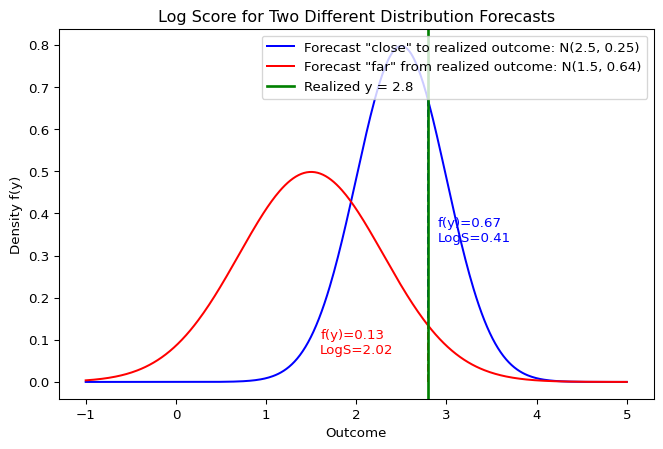
Log Score: Visual Interpretation
The Log Score depends on the height of the density at the realized outcome \(y\). A forecast that assigns higher probability to the realized value receives a better (i.e. lower) score.
Example: Calculating the Log Score
Suppose we forecast that an outcome follows a Normal distribution \(Y \sim \mathcal{N}(\mu=2, \sigma^2=1)\), and the realized value is \(y = 2.5\).
Show the code
import numpy as np
from scipy.stats import norm

mu, sigma = 2, 1
y_obs = 2.5

# Calculate the PDF value at the observed outcome
pdf_val = norm.pdf(y_obs, loc=mu, scale=sigma)
log_score = -np.log(pdf_val)

print(f"PDF value f({y_obs}) = {pdf_val:.4f}")
print(f"Log Score = {log_score:.4f}")
PDF value f(2.5) = 0.3521
Log Score = 1.04393.6 The Continuous Ranked Probability Score (CRPS)
The CRPS measures the “distance” between the forecast’s cumulative distribution function (CDF) and the empirical CDF of the outcome.
We identify each predictive distribution with its CDF, writing \(Y\sim F\) and \(F(z)=\Pr(Y\le z)\) interchangeably.
Definition: For a forecast with CDF \(F\) and a realized outcome \(y\):
\[\text{CRPS}(F, y) = \int_{-\infty}^{\infty} [F(z) - \mathbf{1}\{z \geq y\}]^2 dz\]
where \(\mathbf{1}\{z \geq y\}\) is the Heaviside step function, the CDF of a degenerate predictive distribution that places all probability mass at the realized outcome \(y\).
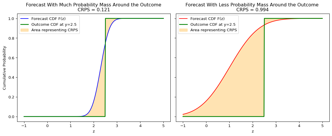
Visual Interpretation
The CRPS measures the squared difference between the forecast CDF, \(F(z)\), and the empirical CDF of the outcome, which is a step function at \(y\). If the forecast places probability mass near the realization, the shaded area is smaller and the CRPS is better (i.e. lower).
Intuition:
- It generalizes the Mean Absolute Error (MAE) to probabilistic forecasts. If the forecast is a single point, the CRPS reduces to the MAE. Even though it may not be intuitive at first sight given the square inside the integral, one can rewrite the CRPS as (Gneiting and Raftery 2007), \[ CRPS(F,y) = \mathbb{E} |X-y| - \frac{1}{2} \mathbb{E} |X-X'| \quad X,X'\stackrel{iid}{\sim}F. \]
- It considers both the location and the spread of the forecast distribution.
- It can be computed even if you only have samples from the forecast distribution, without needing an explicit density function.
Why CRPS Reduces to MAE for a Point Forecast
If the forecast distribution is degenerate at a point forecast \(\hat y\), then \(X=\hat y\) and \(X'=\hat y\) with probability one. In the representation above,
\[ \mathbb{E}|X-y|=|\hat y-y|, \qquad \mathbb{E}|X-X'|=|\hat y-\hat y|=0. \]
Therefore
\[ \text{CRPS}(F,y)=|\hat y-y|, \]
which is exactly the absolute error.
Examples and Computation
For many standard distributions, the CRPS has a closed-form solution.
When no convenient closed form is available, the sample representation makes CRPS useful in simulation-based forecasting. If \(X_1,\ldots,X_M\) are Monte Carlo draws from the predictive distribution, the expectations in the representation above can be approximated by sample averages. This is especially practical when the model can simulate forecast paths but the predictive density or CDF is analytically inconvenient.
For a Normal Distribution: If the forecast is \(F = \mathcal{N}(\mu, \sigma^2)\), the CRPS is:
\[\text{CRPS}(\mathcal{N}(\mu, \sigma^2), y) = \sigma\left[z\left(2\Phi(z) - 1\right) + 2\phi(z) - \frac{1}{\sqrt{\pi}}\right]\]
where \(z = \frac{y - \mu}{\sigma}\), \(\Phi\) is the standard normal CDF, and \(\phi\) is the standard normal PDF.
More closed-form expressions can be found in Jordan, Krüger, and Lerch (2019).
Example: Calculating the CRPS
Using the same forecast \(Y \sim \mathcal{N}(\mu=2, \sigma^2=1)\) and outcome \(y = 2.5\) as above for the log score:
Show the code
# Using the properscoring library for convenience
# pip install properscoring
import properscoring as ps

mu, sigma = 2, 1
y_obs = 2.5

crps_score = ps.crps_gaussian(y_obs, mu=mu, sig=sigma)
print(f"CRPS Score = {crps_score:.4f}")
CRPS Score = 0.33143.7 Comparing LogS vs. CRPS
Both are strictly proper scoring rules, but they have different sensitivities.
| Aspect | Logarithmic Score (LogS) | Continuous Ranked Probability Score (CRPS) |
|---|---|---|
| Input Required | Forecast PDF, \(f(y)\) | Forecast CDF, \(F(y)\) (or samples) |
| Sensitivity | sensitive to tail performance; one bad miss can dominate the average score. | Less sensitive to outliers; focuses on the central tendency and overall shape. |
| Numerical Stability | Can be unstable if \(f(y)\) is close to zero. | Generally very stable. |
| Measurement Error Sensitivity | High | Low |
Practical Rule of Thumb
- Use LogS when tail behavior is central and a full predictive density is available.
- Use CRPS when you want a more robust summary of overall distribution quality or when forecasts are naturally available through CDFs or simulation draws.
In macroeconomic and financial forecasting, it is often informative to report both.
Question for Reflection
If a central bank mostly cares about the probability of very high inflation, would you expect LogS and CRPS to reward the same forecast model? Which score is more aligned with tail-sensitive evaluation, and why?
Suggested Answer
Not necessarily. LogS evaluates the density assigned to the realized outcome and can strongly penalize a model that assigns too little probability to rare high-inflation realizations. CRPS integrates CDF errors over the full support and is often less dominated by one extreme realization. Within the two scores introduced in this chapter, LogS is therefore more aligned with tail-sensitive evaluation, while CRPS is more useful as a robust summary of overall distributional accuracy.
3.8 Assessing Calibration with the Probability Integral Transform
Beyond comparing models with scoring rules, we often want to diagnose how a model’s predictive distributions are failing. A powerful tool for this is the Probability Integral Transform (PIT).
The PIT is based on a fundamental statistical result: if a continuous random variable \(Y\) is drawn from a distribution with cumulative distribution function (CDF) \(F\), then the transformed random variable \(U = F(Y)\) follows a Uniform distribution on the interval [0, 1].
In forecasting, we can apply this principle to a sequence of forecasts and outcomes (Francis X. Diebold, Gunther, and Tay 1998). If our model produces a series of predictive CDFs \(F_t\) for outcomes \(y_t\), and if each conditional distribution is correctly specified relative to the forecast-origin information set \(\mathcal{F}_t\), then the resulting PIT sequence \(u_t = F_t(y_t)\) should be i.i.d. Uniform(0, 1), not merely marginally uniform; deviations in either the marginal shape or the serial dependence signal misspecification. In time-series applications, it is useful to distinguish marginal calibration (the unconditional PIT distribution is Uniform(0,1)) from serial independence (the PIT sequence has no predictable dependence): a PIT histogram can look uniform even when the PIT sequence remains autocorrelated. Conditional calibration requires both — the PIT is Uniform(0,1) and independent of \(\mathcal{F}_t\) — so that both the marginal shape is correct and no leftover predictable pattern remains in the PIT sequence.
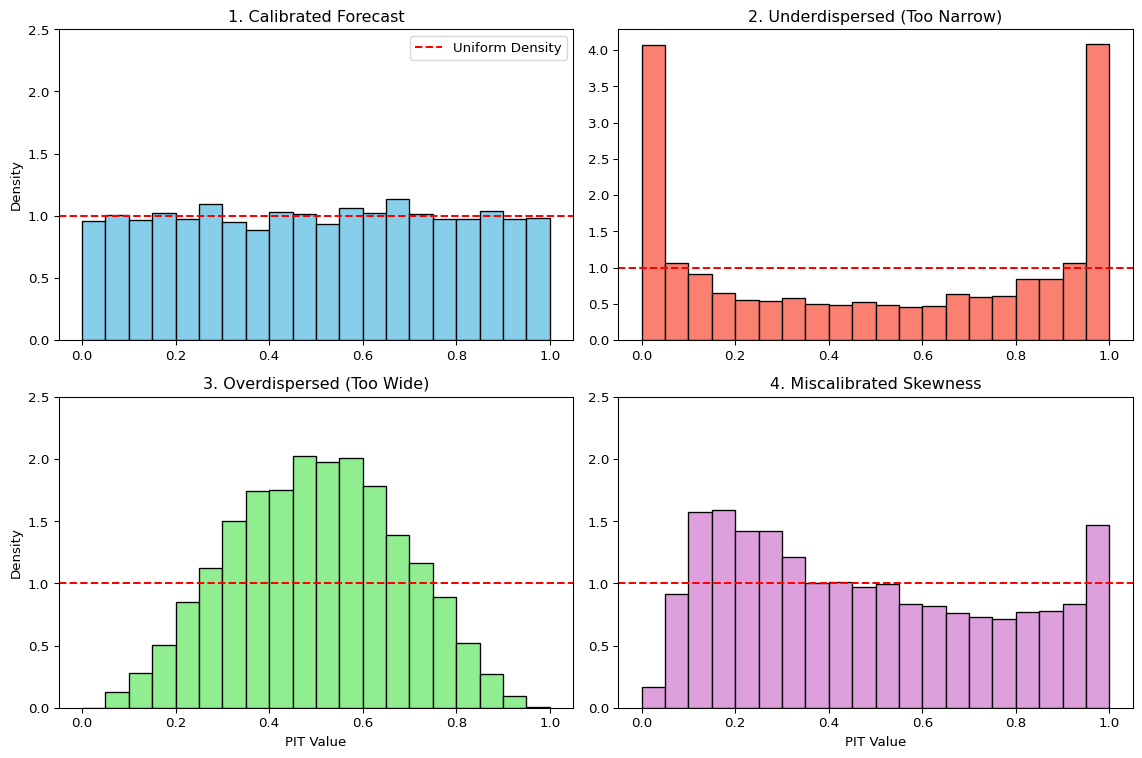
We can visually check this by plotting a histogram of the PIT values. The shape of the histogram reveals systematic biases in the forecast distributions:
- Calibrated Forecasts: If the forecasts are well-calibrated, the PIT histogram will be approximately flat, resembling a uniform distribution.
- Underdispersed Forecasts (Too Narrow): If the forecast distributions are consistently too narrow, the realized outcomes will frequently fall in the tails. This leads to PIT values clustering near 0 and 1, creating a U-shaped histogram. The model is “overconfident” and surprised too often.
- Overdispersed Forecasts (Too Wide): If the forecast distributions are consistently too wide, the realized outcomes will tend to fall in the center of the distributions. This leads to PIT values clustering around 0.5, creating a hump-shaped histogram. The model is “underconfident” in its uncertainty.
- Miscalibrated Skewness: If the histogram is asymmetric or tilted, it indicates a mismatch in skewness. For example, an upward-sloping histogram (more values near 1) suggests the model’s forecasts are not sufficiently right-skewed compared to the outcomes. The model is systematically surprised by large positive outcomes.
The PIT histogram complements scoring rules: scoring rules rank models, PIT histograms diagnose why a model’s predictive distributions are deficient. For dependent data, the PIT should be paired with serial-dependence diagnostics on the PIT sequence; the broader distinction between marginal and conditional coverage reappears in the chapter on conformal prediction.
3.9 Connection to Information Theory
Proper scoring rules connect directly to entropy and cross-entropy from the Information Theory chapter. The link is most direct for the Logarithmic Score.
Let’s assume there is a true, underlying data-generating distribution with density \(p(y)\), and our model produces a forecast distribution with density \(q(y)\).
The Log Score for a single observation \(y\) is:
\[\text{LogS}(q, y) = -\log q(y)\]
To evaluate the quality of our forecasting model \(q\) in general, we consider its expected score under the true distribution \(p\):
\[ \mathbb{E}_{Y \sim p}[\text{LogS}(q, Y)] = \mathbb{E}_{Y \sim p}[-\log q(Y)] = -\int p(y) \log q(y) \,dy \]
This expression is exactly the definition of cross-entropy \(\mathbb{H}_{ce}(p, q)\) between the true distribution \(p\) and the forecast distribution \(q\).
3.10 Minimizing Log Score is Minimizing KL Divergence
Recall the fundamental relationship from information theory:
\[ \underbrace{\mathbb{H}_{ce}(p, q)}_{\text{Expected Log Score}} = \underbrace{\mathbb{H}(p)}_{\text{Entropy of True Process}} + \underbrace{D_{\text{KL}}(p \parallel q)}_{\text{KL Divergence}} \]
This identity decomposes the expected log score into two pieces:
- Entropy \(\mathbb{H}(p)\): the irreducible uncertainty in the true data-generating process. It is the best possible average score, achieved when \(q=p\).
- KL Divergence \(D_{\text{KL}}(p \parallel q)\): the extra loss incurred because \(q\) differs from \(p\). Since \(D_{\text{KL}} \geq 0\), this term is the room for improvement (closely related to the MLE-as-KL discussion).
Implication
Minimizing the average Logarithmic Score is equivalent to minimizing the KL divergence between the model’s predictive distribution \(q\) and the true data-generating distribution \(p\). This is the theoretical foundation for using the Log Score in model selection and evaluation.
Advanced: CRPS and Generalized Entropy
CRPS also admits an interpretation in terms of a generalized entropy. For a forecast CDF \(G\) and true CDF \(F\), the CRPS is
\[\text{CRPS}(G,y)=\int_{-\infty}^{\infty}\big(G(z)-\mathbf{1}\{z \geq y\}\big)^2\,dz.\]
Taking expectation under \(Y \sim F\),
\[ \begin{aligned} \mathbb{E}_{Y\sim F}[\text{CRPS}(G,Y)] &= \int \mathbb{E}\big[(G(z)-\mathbf{1}\{z \geq Y\})^2\big]\,dz \\ &= \int (G(z)-F(z))^2\,dz + \underbrace{\int F(z)(1-F(z))\,dz}_{\mathbb H_{\text{CRPS}}(F)}. \end{aligned} \]
where we used \(\mathbb E[\mathbf{1}\{z \geq Y\}]=F(z)\) and \(\operatorname{Var}(\mathbf{1}\{z \geq Y\})=F(z)(1-F(z))\).
- The term \(\mathbb H_{\text{CRPS}}(F)=\int F(z)(1-F(z))\,dz\) is the generalized “CRPS entropy” of \(F\).
- The excess risk \[D_{\text{CRPS}}(F,G)=\int_{-\infty}^{\infty} (F(z)-G(z))^2\,dz\] is the Cramér–von Mises distance, showing CRPS is strictly proper (minimized at \(G(x)=F(x)\) for all \(x\)).
Equivalent representation:
\[\mathbb H_{\text{CRPS}}(F)=\tfrac{1}{2}\,\mathbb{E}|X-X'|,\quad X,X'\stackrel{iid}{\sim}F,\]
and
\[\text{CRPS}(F,y)=\mathbb{E}|X-y|-\tfrac{1}{2}\mathbb{E}|X-X'| \quad X,X'\stackrel{iid}{\sim}F.\]
The last expression can be used to define a multivariate CRPS analogue called “Energy Score”.
3.11 Beyond LogS and CRPS
Note
- Energy Score for multivariate distributions Székely (2003)
- Diebold-Mariano tests for comparing forecast performance (Francis X. Diebold and Mariano 1995) and the conditional predictive-ability extension of Giacomini and White (2006), which accommodates time-varying or estimated forecasting models and is the standard reference in real-time forecast evaluation
- Quantile scores for specific percentiles of interest (Gneiting and Raftery 2007)
3.12 Empirical Application: GDP Growth Density Forecasts
The tools introduced in this chapter — LogS, CRPS, and PIT histograms — are most informative when applied to competing density forecasts on the same data. We use the same FRED-QD macro panel that appears in the tree chapters. The target is annualized one-step-ahead real GDP growth, and the predictors are five lagged macro and financial variables: lagged GDP growth, inflation, term spread, log VIX, and the unemployment rate.1
Readers who have not yet worked through the random forests chapter only need the following idea for this application: a regression forest is a non-parametric ensemble method which combines multiple predictions into one. We use the following notion in this section: - A mean forest predicts the conditional mean of the target variable given the predictors. - A variance forest predicts the conditional variance of the target variable given the predictors.
We compare three density forecasts, all Gaussian. The AR(1) baseline sets the point forecast to a least-squares AR(1) in lagged GDP growth and the variance to the expanding in-sample residual variance — a quantity that stays roughly constant once enough data are available. The heteroskedastic random forest (in-sample) uses two forests: a mean forest that predicts the conditional mean from all five predictors, and a variance forest that regresses the squared in-sample residuals of the first forest on the same predictors. This two-model construction is analogous to specifying a mean equation and a variance equation separately as, for example, done in GARCH models. The heteroskedastic random forest (OOB) uses the same architecture but feeds the variance forest squared out-of-bag residuals from the mean forest instead.2 We deliberately include both heteroskedastic variants because the two differ only in one design choice — how the residuals fed to the variance forest are produced — and that single choice will turn out to determine whether the model beats or loses to the AR(1) baseline.
All three models are evaluated on the last 25% of the sample — the same test window used in the tree chapters.
Show the code
import numpy as np
import pandas as pd
import matplotlib.pyplot as plt
from scipy.stats import norm
from sklearn.linear_model import LinearRegression
from sklearn.ensemble import RandomForestRegressor
import properscoring as ps

raw = pd.read_csv("data/fred_qd_current.csv")
fred_qd = raw.iloc[2:].copy()
fred_qd["sasdate"] = pd.to_datetime(fred_qd["sasdate"])
for col in fred_qd.columns:
    if col != "sasdate":
        fred_qd[col] = pd.to_numeric(fred_qd[col], errors="coerce")
fred_qd = fred_qd.sort_values("sasdate").reset_index(drop=True)

gdp_growth  = 400 * np.log(fred_qd["GDPC1"]).diff()
inflation   = 400 * np.log(fred_qd["CPIAUCSL"]).diff()
term_spread = fred_qd["GS10"] - fred_qd["TB3MS"]
log_vix     = np.log(fred_qd["VIXCLSx"])

macro = pd.DataFrame({
    "date":        fred_qd["sasdate"].shift(-1),  # target quarter (date of y)
    "y":           gdp_growth.shift(-1),
    "gdp_lag1":    gdp_growth,
    "infl_lag1":   inflation,
    "spread_lag1": term_spread,
    "vix_lag1":    log_vix,
    "unrate_lag1": fred_qd["UNRATE"],
}).dropna().reset_index(drop=True)

feature_cols = ["gdp_lag1", "infl_lag1", "spread_lag1", "vix_lag1", "unrate_lag1"]
split = int(len(macro) * 0.75)

logs_ar, logs_rf, logs_oob = [], [], []
crps_ar, crps_rf, crps_oob = [], [], []
pit_ar,  pit_rf,  pit_oob  = [], [], []
all_dates = []

for t in range(split, len(macro)):
    X_tr = macro.iloc[:t][feature_cols].values
    y_tr = macro.iloc[:t]["y"].values
    X_t  = macro.iloc[t][feature_cols].values.reshape(1, -1)
    y_t  = float(macro.iloc[t]["y"])

    # AR(1): univariate (only gdp_lag1), expanding in-sample mean and constant variance
    ar_X = macro.iloc[:t][["gdp_lag1"]].values
    ar_model = LinearRegression().fit(ar_X, y_tr)
    mu_ar  = ar_model.predict([[macro.iloc[t]["gdp_lag1"]]])[0]
    sig_ar = float(np.std(y_tr - ar_model.predict(ar_X), ddof=1))

    # Heteroskedastic RF (in-sample residuals): mean forest + variance forest
    rf_mean = RandomForestRegressor(n_estimators=400, max_features="sqrt", random_state=42)
    rf_mean.fit(X_tr, y_tr)
    mu_rf       = rf_mean.predict(X_t)[0]
    sq_resid_in = (y_tr - rf_mean.predict(X_tr)) ** 2
    rf_var_in   = RandomForestRegressor(n_estimators=400, max_features="sqrt", random_state=42)
    rf_var_in.fit(X_tr, sq_resid_in)
    sig_rf  = float(np.sqrt(np.clip(rf_var_in.predict(X_t)[0], 1e-6, None)))

    # Heteroskedastic RF (OOB residuals): same architecture, but variance forest
    # is trained on squared OOB residuals from the mean forest
    rf_mean_oob = RandomForestRegressor(n_estimators=400, max_features="sqrt",
                                        bootstrap=True, oob_score=True, random_state=42)
    rf_mean_oob.fit(X_tr, y_tr)
    mu_oob       = rf_mean_oob.predict(X_t)[0]
    sq_resid_oob = (y_tr - rf_mean_oob.oob_prediction_) ** 2
    rf_var_oob   = RandomForestRegressor(n_estimators=400, max_features="sqrt", random_state=42)
    rf_var_oob.fit(X_tr, sq_resid_oob)
    sig_oob = float(np.sqrt(np.clip(rf_var_oob.predict(X_t)[0], 1e-6, None)))

    logs_ar.append(-norm.logpdf(y_t, mu_ar, sig_ar))
    logs_rf.append(-norm.logpdf(y_t, mu_rf, sig_rf))
    logs_oob.append(-norm.logpdf(y_t, mu_oob, sig_oob))
    crps_ar.append(ps.crps_gaussian(y_t, mu=mu_ar, sig=sig_ar))
    crps_rf.append(ps.crps_gaussian(y_t, mu=mu_rf, sig=sig_rf))
    crps_oob.append(ps.crps_gaussian(y_t, mu=mu_oob, sig=sig_oob))
    pit_ar.append(float(norm.cdf(y_t, mu_ar, sig_ar)))
    pit_rf.append(float(norm.cdf(y_t, mu_rf, sig_rf)))
    pit_oob.append(float(norm.cdf(y_t, mu_oob, sig_oob)))
    all_dates.append(macro.iloc[t]["date"])

test_dates = pd.to_datetime(all_dates)
covid_start = pd.Timestamp("2020-04-01")
covid_end   = pd.Timestamp("2020-06-30")

fig, axes = plt.subplots(2, 1, figsize=(11, 6), sharex=True)
for ax, vals_ar, vals_rf, vals_oob, ylabel in zip(
    axes,
    [logs_ar, crps_ar],
    [logs_rf, crps_rf],
    [logs_oob, crps_oob],
    ["LogS (lower = better)", "CRPS (lower = better)"],
):
    ax.axvspan(covid_start, covid_end, color="0.85", label="2020Q2")
    ax.plot(test_dates, vals_ar,  color="C1", linewidth=1.2, label="AR(1) baseline")
    ax.plot(test_dates, vals_rf,  color="C3", linewidth=1.2, label="RF (in-sample)")
    ax.plot(test_dates, vals_oob, color="C0", linewidth=1.2, label="RF (OOB)")
    ax.set_ylabel(ylabel)
    ax.legend(frameon=False)
    ax.grid(True, alpha=0.25)

axes[1].set_xlabel("Quarter")
plt.tight_layout()
plt.show()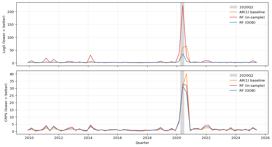
The top panel of Figure 3.5 shows LogS over time. All three models register a sharp spike in 2020Q2, the quarter in which GDP fell by roughly 30 percent annualized. Because LogS evaluates the density at the realized outcome, a single quarter that falls far into the left tail — where any Gaussian forecast assigns near-zero probability — can inflate the average LogS dramatically. The spike is by far the largest for the in-sample RF: its variance forest had been predicting a small conditional variance going into 2020, so the resulting density at \(-32.8\%\) is essentially zero. The OOB RF’s variance forecast is on a more realistic scale, so its 2020Q2 spike is smaller; the AR(1) sits in between. The bottom panel plots CRPS over the same period. All three models deteriorate in 2020Q2, but more moderately than under LogS: CRPS integrates the CDF discrepancy over all values rather than evaluating density at one point, so it is less sensitive to a single catastrophic miss.
Show the code
fig, axes = plt.subplots(2, 2, figsize=(11, 8))
ax_bar, ax_ar, ax_rf, ax_oob = axes.flatten()

# Average scores bar chart
labels = ["AR(1)", "RF\n(in-sample)", "RF\n(OOB)"]
x = np.arange(len(labels))
width = 0.35
score_colors = ["C1", "C3", "C0"]
ax_bar.bar(x - width/2,
           [np.mean(logs_ar), np.mean(logs_rf), np.mean(logs_oob)],
           width, label="LogS", color=score_colors, alpha=0.85)
ax_bar.bar(x + width/2,
           [np.mean(crps_ar), np.mean(crps_rf), np.mean(crps_oob)],
           width, label="CRPS", color=score_colors, alpha=0.45, hatch="//")
ax_bar.set_xticks(x)
ax_bar.set_xticklabels(labels)
ax_bar.set_ylabel("Average score (lower = better)")
ax_bar.set_title("Average Scores")
ax_bar.legend(frameon=False)
ax_bar.grid(True, axis="y", alpha=0.3)

# PIT histograms
bins = np.linspace(0, 1, 16)
for ax, pit_vals, title, color in zip(
    [ax_ar, ax_rf, ax_oob],
    [pit_ar, pit_rf, pit_oob],
    ["PIT: AR(1) baseline", "PIT: RF (in-sample)", "PIT: RF (OOB)"],
    ["C1", "C3", "C0"],
):
    ax.hist(pit_vals, bins=bins, density=True, color=color, edgecolor="white", alpha=0.8)
    ax.axhline(1.0, color="red", linestyle="--", linewidth=1, label="Uniform")
    ax.set_xlabel("PIT value")
    ax.set_ylabel("Density")
    ax.set_title(title)
    ax.set_ylim(0, 5.2)
    ax.legend(frameon=False)
    ax.grid(True, alpha=0.25)

plt.tight_layout()
plt.show()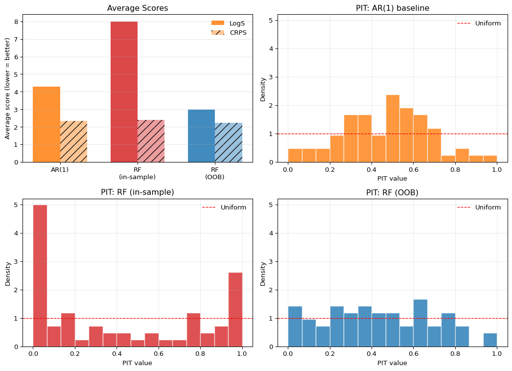
The top-left panel of Figure 3.6 reports average scores. The ranking is striking. The in-sample heteroskedastic RF loses badly to the AR(1) baseline on both LogS and CRPS — the gap is especially large for LogS, where the small predicted variance produces near-zero density at the COVID realization. The OOB heteroskedastic RF wins on both LogS and CRPS over the same test window. The two RFs differ only in whether the variance forest is trained on in-sample or out-of-bag residuals, yet that single design choice flips the ranking against the baseline.
The PIT histograms in the remaining panels diagnose why. The AR(1) PIT is mildly hump-shaped: with its constant in-sample residual variance, it is, if anything, slightly overdispersed in the relatively calm post-2009 period. The in-sample RF PIT is sharply U-shaped, with very large mass near \(0\) and \(1\) — the classic signature of an underdispersed predictive distribution. This is the variance-forest construction biting back: training the variance equation on in-sample mean-forest residuals systematically underestimates the conditional variance, so the resulting Gaussian densities are too narrow and realizations land in the tails far more often than a calibrated forecast would imply. The OOB RF PIT is the flattest of the three, with no edge spikes and a mostly even spread across the unit interval. Replacing in-sample residuals with out-of-bag residuals removes the overfit and gives the variance forest a realistic target to learn.
This is the central pedagogical point of the application. A flexible ML model that adds a learned variance equation does not automatically beat a simple AR(1) — if you train the variance equation on residuals that the mean equation has already overfit, you will lose to a model with no variance equation at all. The PIT histogram diagnoses this failure mode directly. But once that single design issue is fixed, the same architecture that lost on both scores now wins on both. The lesson is not that ML is too dangerous to use for density forecasting; it is that the diagnostics in this chapter — proper scoring rules together with calibration plots — are precisely what lets you tell a working ML pipeline apart from one that is broken in a way you would otherwise miss.
Question for Reflection
Both models use a Gaussian predictive distribution. How would you expect the PIT histogram to change if GDP growth were right-skewed in the test period? Which panel in Figure 3.4 corresponds to that pattern, and what model modification would address it?
Suggested Answer
Right-skewed realized outcomes relative to a symmetric Gaussian forecast would produce an upward-sloping PIT histogram: more realizations fall in the right tail than the Gaussian allocates probability to, pushing PIT values toward 1. This corresponds to the miscalibrated-skewness panel in Figure 3.4. The natural modification is to replace the Gaussian with a distribution that supports negative outcomes and allows for skewness, such as a skew-normal or skew-\(t\), or to fit a distributional neural network that learns the conditional skewness from the predictors directly.
3.13 Summary
Key Takeaways
- Distribution forecasts are essential when economic or financial decisions depend on uncertainty, tail risk, or the full conditional distribution.
- Proper scoring rules are needed because they reward honest reporting of predictive uncertainty rather than only point accuracy.
- LogS is especially useful when tail behavior matters and a full density is available, while CRPS is often more robust and easier to use with CDFs or simulated forecasts.
- PIT histograms complement scoring rules by diagnosing whether forecast distributions are too narrow, too wide, or misspecified in skewness.
- Information theory provides the conceptual foundation: minimizing average LogS is equivalent to minimizing cross-entropy, hence KL divergence up to the irreducible entropy term.
Common Pitfalls
- Ranking models only by point-forecast accuracy when the decision problem depends on the full predictive distribution.
- Treating a good PIT histogram as sufficient evidence that a model is optimal, even when its scoring-rule performance is weak.
- Using LogS without recognizing how strongly it punishes tail misspecification and near-zero assigned density.
- Interpreting CRPS as “just another loss function” rather than a proper scoring rule for full predictive distributions.
- Forgetting that calibration diagnostics must be applied out of sample, not on the estimation sample.
- Building a two-stage density forecast by training a variance model on squared in-sample residuals from a flexible mean model. Overfitting in the mean model deflates the residuals, so the variance model learns an overconfident scale and the resulting Gaussian density becomes sharply underdispersed. Out-of-bag or held-out residuals avoid this leak.
3.14 Exercises
Exercise 3.1: Expected Log Score Under Gaussian Misspecification
Suppose the true predictive distribution is
\[ p(y)=\mathcal{N}(\mu_0,\sigma_0^2), \]
while a forecaster reports the Gaussian predictive density
\[ q(y)=\mathcal{N}(\mu,\sigma^2), \qquad \sigma^2>0. \]
- Show that the logarithmic score for a realized outcome \(y\) can be written as \[ \mathrm{LogS}(q,y)=\frac{1}{2}\log(2\pi\sigma^2)+\frac{(y-\mu)^2}{2\sigma^2}. \]
- Compute the expected log score under the true distribution \(p\) and show that \[ \mathbb{E}_{Y\sim p}[\mathrm{LogS}(q,Y)] = \frac{1}{2}\log(2\pi\sigma^2) +\frac{\sigma_0^2+(\mu_0-\mu)^2}{2\sigma^2}. \]
- Show that the expected log score is minimized at \[ \mu=\mu_0, \qquad \sigma^2=\sigma_0^2. \]
- Explain why this differs from point-forecast evaluation with MSE, where only the conditional mean matters.
Exam level. The exercise formalizes why LogS evaluates the entire predictive distribution, not just its center.
Hint for Part 1
Start from the Gaussian density formula and take minus the logarithm.
Hint for Part 2
Use
\[ \mathbb{E}\big[(Y-\mu)^2\big] = \operatorname{Var}(Y)+\big(\mathbb{E}[Y]-\mu\big)^2. \]
Hint for Part 3
Differentiate the expression from Part 2 first with respect to \(\mu\), then with respect to \(\sigma^2\).
Hint for Part 4
Under squared-error loss, the optimal point forecast is the conditional mean. Under LogS, both location and uncertainty enter the criterion.
Solution
Part 1: Writing the Gaussian Log Score
For a Gaussian predictive density,
\[ q(y)=\frac{1}{\sqrt{2\pi\sigma^2}} \exp\left(-\frac{(y-\mu)^2}{2\sigma^2}\right). \]
Taking minus the logarithm gives
\[ \mathrm{LogS}(q,y) = \frac{1}{2}\log(2\pi\sigma^2)+\frac{(y-\mu)^2}{2\sigma^2}. \]
Part 2: Taking the Expected Log Score
Take expectation under \(Y\sim \mathcal{N}(\mu_0,\sigma_0^2)\):
\[ \mathbb{E}_{Y\sim p}[\mathrm{LogS}(q,Y)] = \frac{1}{2}\log(2\pi\sigma^2)+\frac{1}{2\sigma^2}\mathbb{E}\big[(Y-\mu)^2\big]. \]
Now
\[ \mathbb{E}\big[(Y-\mu)^2\big] = \operatorname{Var}(Y)+(\mathbb{E}[Y]-\mu)^2 = \sigma_0^2+(\mu_0-\mu)^2. \]
Therefore
\[ \mathbb{E}_{Y\sim p}[\mathrm{LogS}(q,Y)] = \frac{1}{2}\log(2\pi\sigma^2) +\frac{\sigma_0^2+(\mu_0-\mu)^2}{2\sigma^2}. \]
Part 3: Optimizing over Mean and Variance
First differentiate with respect to \(\mu\):
\[ \frac{\partial}{\partial \mu} \mathbb{E}_{Y\sim p}[\mathrm{LogS}(q,Y)] = \frac{\mu-\mu_0}{\sigma^2}. \]
So the optimum in \(\mu\) is
\[ \mu=\mu_0. \]
Substituting this into the expected score gives
\[ \frac{1}{2}\log(2\pi\sigma^2)+\frac{\sigma_0^2}{2\sigma^2}. \]
Differentiate with respect to \(\sigma^2\):
\[ \frac{\partial}{\partial \sigma^2} \left( \frac{1}{2}\log(2\pi\sigma^2)+\frac{\sigma_0^2}{2\sigma^2} \right) = \frac{1}{2\sigma^2}-\frac{\sigma_0^2}{2(\sigma^2)^2}. \]
Setting this equal to zero yields
\[ \sigma^2=\sigma_0^2. \]
Hence the expected log score is minimized at the true mean and the true variance.
Part 4: Why LogS Goes Beyond Point Forecasts
Point-forecast evaluation with MSE only asks for the optimal point forecast, which is the conditional mean. It does not reward or penalize the predictive variance at all.
By contrast, LogS evaluates the full predictive density. A forecaster can get the mean right but still be penalized for reporting a variance that is too small or too large. That is why LogS is suitable for distribution forecasts rather than only point forecasts.
Exercise 3.2: Why CRPS Is Proper
Let \(F\) denote the true predictive CDF, let \(G\) denote a forecast CDF, and let \(Y\sim F\). Recall the CRPS:
\[ \mathrm{CRPS}(G,y)=\int_{-\infty}^{\infty}\big(G(z)-\mathbf{1}\{z\ge y\}\big)^2\,dz. \]
- Show that \[ \mathbb{E}_{Y\sim F}[\mathrm{CRPS}(G,Y)] = \int_{-\infty}^{\infty}\left[\big(G(z)-F(z)\big)^2+F(z)\big(1-F(z)\big)\right]\,dz. \]
- Show that the expected CRPS is minimized at \(G=F\).
- Prove that for a point forecast represented by the degenerate CDF \(G(z)=\mathbf{1}\{z\ge \hat y\}\), \[ \mathrm{CRPS}(G,y)=|\hat y-y|. \]
Exam level. The exercise proves propriety and then shows why CRPS reduces to MAE for a degenerate point forecast.
Hint for Part 1
Take expectation inside the integral, expand the square, and use
\[ \mathbb{E}[\mathbf{1}\{z\ge Y\}] = F(z), \qquad \mathbb{E}[\mathbf{1}\{z\ge Y\}^2] = F(z). \]
Hint for Part 2
In the expression from Part 1, only one integral depends on \(G\).
Hint for Part 3
For the degenerate forecast, the integrand is zero on one side of the interval between \(\hat y\) and \(y\), and one on the other side.
Solution
Part 1: Expected CRPS Decomposition
By definition,
\[ \mathrm{CRPS}(G,Y)=\int_{-\infty}^{\infty}\big(G(z)-\mathbf{1}\{z\ge Y\}\big)^2\,dz. \]
Taking expectation under \(Y\sim F\) gives
\[ \mathbb{E}_{Y\sim F}[\mathrm{CRPS}(G,Y)] = \int_{-\infty}^{\infty}\mathbb{E}\Big[\big(G(z)-\mathbf{1}\{z\ge Y\}\big)^2\Big]\,dz. \]
Expand the square:
\[ \big(G(z)-\mathbf{1}\{z\ge Y\}\big)^2 = G(z)^2-2G(z)\mathbf{1}\{z\ge Y\}+\mathbf{1}\{z\ge Y\}. \]
Taking expectations yields
\[ \mathbb{E}\Big[\big(G(z)-\mathbf{1}\{z\ge Y\}\big)^2\Big] = G(z)^2-2G(z)F(z)+F(z). \]
Now add and subtract \(F(z)^2\):
\[ G(z)^2-2G(z)F(z)+F(z)^2+F(z)-F(z)^2. \]
Therefore
\[ \mathbb{E}\Big[\big(G(z)-\mathbf{1}\{z\ge Y\}\big)^2\Big] = \big(G(z)-F(z)\big)^2+F(z)\big(1-F(z)\big). \]
Substituting this into the integral gives
\[ \mathbb{E}_{Y\sim F}[\mathrm{CRPS}(G,Y)] = \int_{-\infty}^{\infty}\big(G(z)-F(z)\big)^2\,dz + \int_{-\infty}^{\infty}F(z)\big(1-F(z)\big)\,dz. \]
Part 2: Propriety of CRPS
The second integral depends only on the true distribution \(F\). So the only term depending on the forecast \(G\) is
\[ \int_{-\infty}^{\infty}\big(G(z)-F(z)\big)^2\,dz, \]
which is nonnegative and equals zero if and only if \(G(z)=F(z)\) for all \(z\). Hence the expected CRPS is minimized at the true forecast distribution \(G=F\).
Part 3: Degenerate Forecasts and Absolute Error
Now let
\[ G(z)=\mathbf{1}\{z\ge \hat y\}. \]
Then
\[ \mathrm{CRPS}(G,y) = \int_{-\infty}^{\infty}\big(\mathbf{1}\{z\ge \hat y\}-\mathbf{1}\{z\ge y\}\big)^2\,dz. \]
If \(\hat y<y\), the integrand equals 1 exactly on the interval \([\hat y,y)\) and 0 elsewhere, so
\[ \mathrm{CRPS}(G,y)=y-\hat y. \]
If \(\hat y>y\), the integrand equals 1 exactly on \([y,\hat y)\), so
\[ \mathrm{CRPS}(G,y)=\hat y-y. \]
Therefore in all cases,
\[ \mathrm{CRPS}(G,y)=|\hat y-y|. \]
So CRPS reduces to the absolute error for a degenerate point forecast.
Exercise 3.3: PIT Under Dispersion Misspecification
Suppose the true distribution is standard normal:
\[ Y\sim \mathcal{N}(0,1). \]
Suppose the forecaster reports the Gaussian predictive CDF
\[ F_\sigma(y)=\Phi\left(\frac{y}{\sigma}\right), \qquad \sigma>0, \]
where \(\Phi\) and \(\phi\) denote the standard normal CDF and PDF.
Define the PIT value by
\[ U=F_\sigma(Y). \]
- Show that for any \(u\in(0,1)\), \[ \mathbb{P}(U\le u)=\Phi\big(\sigma\,\Phi^{-1}(u)\big). \] and differentiate this expression to show that the PIT density is \[ f_U(u) = \sigma\, \frac{\phi\big(\sigma\Phi^{-1}(u)\big)}{\phi\big(\Phi^{-1}(u)\big)}, \qquad 0<u<1. \]
- Show that if \(\sigma=1\), then \(U\sim \mathrm{Uniform}(0,1)\).
- Show that \[ f_U(u)=\sigma\exp\left(\frac{1-\sigma^2}{2}\big(\Phi^{-1}(u)\big)^2\right). \] Use this to explain why the PIT histogram is U-shaped when \(\sigma<1\) and hump-shaped when \(\sigma>1\).
Exam level. This exercise turns the usual PIT intuition into an explicit distributional calculation.
Hint for Part 1
Use that \(\Phi\) is strictly increasing:
\[ U\le u \quad\Longleftrightarrow\quad \Phi\left(\frac{Y}{\sigma}\right)\le u. \]
Differentiate \(\Phi(\sigma \Phi^{-1}(u))\) using the chain rule and
\[ \frac{d}{du}\Phi^{-1}(u)=\frac{1}{\phi(\Phi^{-1}(u))}. \]
Hint for Part 2
Substitute \(\sigma=1\) into the CDF or density from Part 1.
Hint for Part 3
Write
\[ \phi(z)=\frac{1}{\sqrt{2\pi}}e^{-z^2/2} \]
and simplify the ratio.
Solution
Part 1: Deriving the PIT Distribution
Since \(\Phi\) is strictly increasing,
\[ U\le u \quad\Longleftrightarrow\quad \Phi\left(\frac{Y}{\sigma}\right)\le u \quad\Longleftrightarrow\quad \frac{Y}{\sigma}\le \Phi^{-1}(u) \quad\Longleftrightarrow\quad Y\le \sigma \Phi^{-1}(u). \]
Therefore
\[ \mathbb{P}(U\le u)=\mathbb{P}\big(Y\le \sigma\Phi^{-1}(u)\big) = \Phi\big(\sigma\Phi^{-1}(u)\big). \]
Differentiate the CDF:
\[ f_U(u)=\frac{d}{du}\Phi\big(\sigma\Phi^{-1}(u)\big). \]
By the chain rule,
\[ f_U(u) = \phi\big(\sigma\Phi^{-1}(u)\big)\cdot \sigma \cdot \frac{d}{du}\Phi^{-1}(u). \]
Using
\[ \frac{d}{du}\Phi^{-1}(u)=\frac{1}{\phi(\Phi^{-1}(u))}, \]
we obtain
\[ f_U(u) = \sigma\, \frac{\phi\big(\sigma\Phi^{-1}(u)\big)}{\phi\big(\Phi^{-1}(u)\big)}. \]
Part 2: Recovering Uniformity Under Correct Specification
If \(\sigma=1\), then from Part 1
\[ \mathbb{P}(U\le u)=\Phi(\Phi^{-1}(u))=u. \]
So \(U\) has the Uniform\((0,1)\) distribution.
Part 3: Why Dispersion Errors Distort the PIT Histogram
Let \(z=\Phi^{-1}(u)\). Then
\[ f_U(u) = \sigma\frac{\phi(\sigma z)}{\phi(z)} = \sigma\frac{\frac{1}{\sqrt{2\pi}}e^{-\sigma^2 z^2/2}} {\frac{1}{\sqrt{2\pi}}e^{-z^2/2}} = \sigma\exp\left(\frac{1-\sigma^2}{2}z^2\right). \]
Hence
\[ f_U(u)=\sigma\exp\left(\frac{1-\sigma^2}{2}\big(\Phi^{-1}(u)\big)^2\right). \]
If \(\sigma<1\), then \(1-\sigma^2>0\), so the exponent is positive and grows with \(|\Phi^{-1}(u)|\). Therefore the density is large near the edges \(u\approx 0\) and \(u\approx 1\), which gives a U-shaped PIT histogram. This corresponds to an underdispersed forecast.
If \(\sigma>1\), then \(1-\sigma^2<0\), so the density is damped in the tails and relatively larger near the center. This gives a hump-shaped PIT histogram, corresponding to an overdispersed forecast.
3.15 References
Diebold, Francis X., Todd A. Gunther, and Anthony S. Tay. 1998. “Evaluating Density Forecasts with Applications to Financial Risk Management.” International Economic Review 39 (4): 863–83. https://doi.org/10.2307/2527342.
Diebold, Francis X, and Robert S Mariano. 1995. “Comparing predictive accuracy.” Journal of Business and Economic Statistics 13 (3): 253–63. https://doi.org/10.1080/07350015.1995.10524599.
Giacomini, Raffaella, and Halbert White. 2006. “Tests of Conditional Predictive Ability.” Econometrica 74 (6): 1545–78. https://doi.org/10.1111/j.1468-0262.2006.00718.x.
Gneiting, Tilmann, and Adrian E. Raftery. 2007. “Strictly proper scoring rules, prediction, and estimation.” Journal of the American Statistical Association 102 (477): 359–78. https://doi.org/10.1198/016214506000001437.
Jordan, Alexander, Fabian Krüger, and Sebastian Lerch. 2019. “Evaluating probabilistic forecasts with scoringRules.” Journal of Statistical Software 90 (12): 1–37. https://doi.org/10.18637/jss.v090.i12.
Székely, Gábor J. 2003. “\(E\)-Statistics: The Energy of Statistical Samples.” Technical Report 03-05. Bowling Green State University, Department of Mathematics; Statistics.
Footnotes
This is a pedagogical final-vintage FRED-QD example. A full real-time evaluation would need to account for data revisions and publication lags.↩︎
All forests are re-estimated at each forecast origin using only data available at that point, so there is no look-ahead. The in-sample variant trains the variance forest on \(\hat\varepsilon_t^2 = (y_t - \hat\mu_t)^2\), where \(\hat\mu_t\) comes from the mean forest fit on the same training window. Because random forests fit the training data closely, these in-sample residuals understate the true conditional variance and the variance forest predicts overconfident scales. The OOB variant replaces \(\hat\mu_t\) with the out-of-bag prediction from the mean forest — for each training observation, the average prediction across only those trees that did not see it during bootstrap. OOB residuals are not affected by same-sample overfitting and therefore give the variance forest a more realistic conditional-scale target than in-sample residuals (in dependent macro data they are not honest real-time forecast errors, but they are still substantially less overfit). The
np.clip(..., 1e-6, None)guard keeps the predicted variance strictly positive, which preventsLogSfrom blowing up at near-zero leaf averages.↩︎