Under active development. A stable version is expected in November 2026. Feedback is welcome by email or via GitHub issues.
Show the code
import matplotlib.pyplot as pltimport numpy as np# Create figurefig, ax = plt.subplots(1, 1, figsize=(10, 6))# Create a simple tree structureax.text(0.5, 0.9, 'Root Node\n(All Data)', ha='center', va='center', bbox=dict(boxstyle="round,pad=0.3", facecolor='lightblue'), fontsize=12, fontweight='bold')# Left branchax.text(0.25, 0.6, 'Feature X₁ < 5?', ha='center', va='center', bbox=dict(boxstyle="round,pad=0.3", facecolor='lightgreen'), fontsize=10)# Right branch ax.text(0.75, 0.6, 'Feature X₂ < 3?', ha='center', va='center', bbox=dict(boxstyle="round,pad=0.3", facecolor='lightgreen'), fontsize=10)# Terminal nodesax.text(0.15, 0.3, 'Prediction:\nClass A', ha='center', va='center', bbox=dict(boxstyle="round,pad=0.3", facecolor='salmon'), fontsize=10)ax.text(0.35, 0.3, 'Prediction:\nClass B', ha='center', va='center', bbox=dict(boxstyle="round,pad=0.3", facecolor='salmon'), fontsize=10)ax.text(0.65, 0.3, 'Prediction:\nClass C', ha='center', va='center', bbox=dict(boxstyle="round,pad=0.3", facecolor='salmon'), fontsize=10)ax.text(0.85, 0.3, 'Prediction:\nClass A', ha='center', va='center', bbox=dict(boxstyle="round,pad=0.3", facecolor='salmon'), fontsize=10)# Draw arrowsarrows = [ ((0.5, 0.85), (0.25, 0.65)), # Root to left ((0.5, 0.85), (0.75, 0.65)), # Root to right ((0.25, 0.55), (0.15, 0.35)), # Left to terminal ((0.25, 0.55), (0.35, 0.35)), # Left to terminal ((0.75, 0.55), (0.65, 0.35)), # Right to terminal ((0.75, 0.55), (0.85, 0.35)), # Right to terminal]for start, end in arrows: ax.annotate('', xy=end, xytext=start, arrowprops=dict(arrowstyle='->', lw=2, color='black'))ax.set_xlim(0, 1)ax.set_ylim(0, 1)ax.axis('off')plt.tight_layout()plt.show()
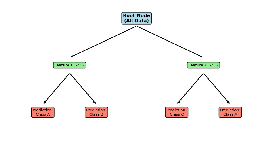
Figure 8.1: Example of a decision tree structure
8.1 Mathematical Framework
Decision trees are part of the supervised learning goal part of machine learning which means: Learn about the relationship \(f\) between \(\mathbf{y}\) and \(\mathbf{x}\) using training sample \(\{(\mathbf{x}_i, y_i)\}_{i=1}^N\) to get an estimate \(\hat{f}\) of \(f\).
For comparison, a feed-forward neural network with \(L\) layers can be written as a composition of functions:
Components of a tree: root node, decision nodes, and leaf nodes
A tree consists of: - Root node: Starting point containing all data - Internal nodes: Decision points that split the data - Leaf nodes: Terminal nodes that contain the final predictions
where \(\hat{y}_{R_j}\) is the mean response for training observations in the \(j\)-th box.
Computational Challenge
Unfortunately, it is computationally infeasible to consider every possible partition of the feature space into \(J\) boxes.
Solution: Use a top-down, greedy approach called recursive binary splitting:
Top-down: Begin at the top of the tree and successively split the predictor space
Greedy: At each step, make the best split at that moment, without looking ahead
10.4 Node Splitting Process
Node splitting diagram showing how a parent region R is split into left and right child regions
Splitting Mechanism
In each decision node, we: - Choose a splitting feature\(x_j\) - Choose a threshold value\(s\) - Create two regions: - \(R_\ell(j,s) = \{\mathbf{x} | x_j \leq s\}\) (left child) - \(R_r(j,s) = \{\mathbf{x} | x_j > s\}\) (right child)
Algorithm Details
First split: Select predictor \(x_j\) and cutpoint \(s\) (across all \(j\) and \(s\)) that leads to the greatest reduction in RSS when splitting into \(\{\mathbf{x} | x_j < s\}\) and \(\{\mathbf{x} | x_j \geq s\}\)
Subsequent splits: Repeat the process, looking for the best predictor and cutpoint to split one of the existing regions
Continue: Until a stopping criterion is reached (e.g., no region contains more than a fixed number of observations)
11 Trees for Classification
Classification Tree Example
Example of a classification tree for mortgage approval decisions
Visualization of Classification Regions
Scatter plot showing classification regions for blue vs red classes
Scatter plot of classes “blue” vs “red” depending on features \(x_1\) and \(x_2\) with exemplary segmentation into boxes.
where \(\hat{y}_{R_j} = \frac{1}{|R_j|} \sum_{x_i \in R_j} y_i\)
Classification trees: Need a different “cost measure” for class assignment. Since the response is categorical, MSE is no longer appropriate — we need a measure of node impurity that captures how “mixed” the class labels are within a region.
Node Impurity and Entropy
Recall from our Information Theory chapter that entropy quantifies the uncertainty in a distribution. For a node with empirical class frequency \(\hat{\pi}\) (the proportion of class “1” observations), the entropy is exactly the Bernoulli entropy we studied earlier:
This is maximized at \(\hat{\pi} = 0.5\) (maximum uncertainty, the node is an even mix of classes) and zero at \(\hat{\pi} \in \{0, 1\}\) (the node is pure). A good split should produce child nodes with lower entropy than the parent — i.e., the split should reduce uncertainty about the class label.
Information Gain
The criterion for choosing a split is information gain, defined as the reduction in entropy from the parent node to the weighted average entropy of the child nodes:
where \(n_\ell, n_r\) are the sample sizes in the left and right child nodes after splitting feature \(x_j\) at threshold \(s\). The greedy algorithm selects the \((j, s)\) pair that maximizes information gain.
Connection to KL divergence
Information gain can be interpreted as a weighted sum of KL divergences between each child’s class distribution and the parent’s class distribution. Maximizing information gain is therefore equivalent to finding the split that makes the children’s distributions most different from the parent — exactly the idea of “learning something new” from the split.
Binary Classification Trees
Putting this together, the objective for growing a classification tree is to find boxes \(R_1, \dots, R_J\) that minimize the total entropy across all \(J\) terminal nodes:
where \(\hat{\pi}_{R_j} = \frac{1}{|R_j|} \sum_{x_i \in R_j} y_i\) is the empirical frequency of class “1” in region \(R_j\).
Other impurity measures
In practice, the Gini impurity\(G(\hat{\pi}) = 2\hat{\pi}(1-\hat{\pi})\) is often used as an alternative to entropy. Both are concave functions of \(\hat{\pi}\) that are maximized at 0.5 and zero at 0 and 1. In most applications the choice between Gini and entropy makes little practical difference, but entropy has the advantage of a direct information-theoretic interpretation.
12 When to Stop Growing the Tree?
12.1 The Overfitting Problem
Trees can easily overfit if grown too deep. The following figures illustrate how tree depth affects model complexity:
Goal: Avoid overfitting, which can easily happen with a fully grown or large tree
Methods to limit tree size a priori: 1. Minimum sample size: Require a minimum number of observations in each leaf 2. Maximum depth: Impose a maximum depth of the tree
12.3 Hyperparameters
The main hyperparameters for decision trees are: 1. Minimum sample size at each leaf 2. Maximum depth of the tree
These need to be tuned using techniques like cross-validation.
12.4 Alternative Approaches
Instead of trying to find the optimal single tree, this course focuses on two alternatives: - Boosting: Combining simple trees sequentially - Random forests: Combining deep trees via averaging
13 Advantages and Disadvantages of Trees
13.1 Advantages
Interpretability: Trees are very easy to explain to people - even easier than linear regression!
Visualization: Trees can be displayed graphically and are easily interpreted even by non-experts (when they are small)
Intuitive: They mirror human decision-making processes
13.2 Disadvantages
Poor accuracy: Trees generally do not have the same level of predictive accuracy as other regression and classification approaches
Instability: Small changes in data can lead to very different trees
Overfitting: Prone to overfitting, especially when grown deep